Figures

A handful of figures trying out different functions within ggplot.

hide

liz <-  read_csv(here::here("lizards.csv"))

hide

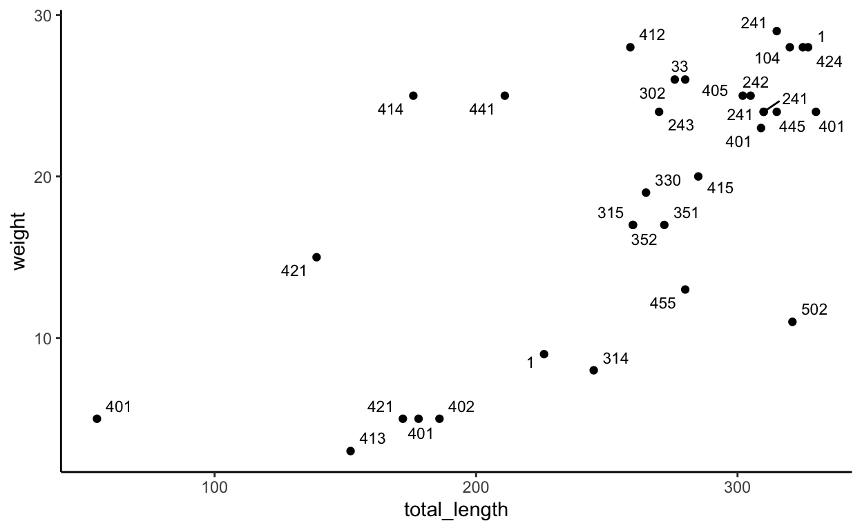
ww_liz <- liz %>% 
  filter(common_name == "western whiptail", site == "sand")

ggplot(ww_liz, aes(x = total_length, y = weight)) +
  geom_point() +
  theme_classic() +
  geom_text_repel(aes(label = toe_num), size = 3, max.overlaps = 20)

hide

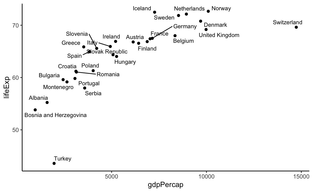
data <- gapminder %>% 
  filter(continent == "Europe", year == 1952)

ggplot(data, aes(x = gdpPercap, y = lifeExp)) +
  geom_point() +
  geom_text_repel(aes(label = country), size =  3) +
  theme_classic()

hide

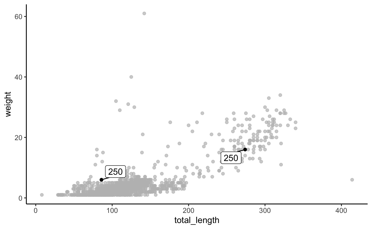
p <- ggplot(liz, aes(x = total_length, y = weight)) +
  geom_point()

p + gghighlight(toe_num == 250, label_key = toe_num) + 
  theme_classic()

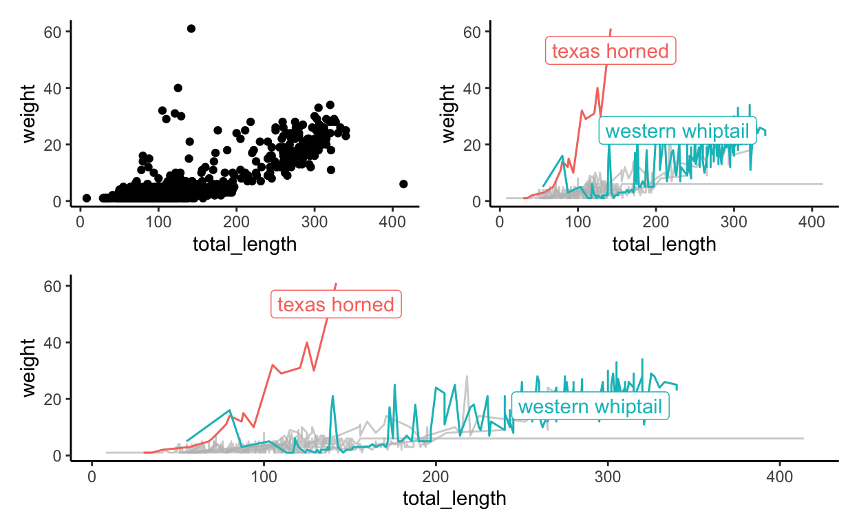
hide

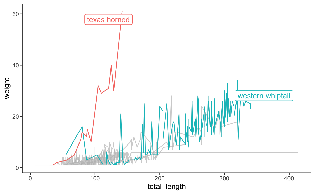
q <- ggplot(liz, aes(x = total_length, y = weight)) +
  geom_line(aes(color = common_name)) +
  gghighlight(max(weight) > 30) +
  theme_classic()

q

hide

(p | q) / q & theme_classic()

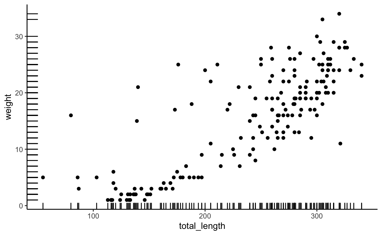
hide

whiptails <- liz %>% 
  filter(common_name == "western whiptail") %>% 
  drop_na(total_length, weight)

ggplot(data = whiptails, aes(x = total_length, y = weight)) +
  geom_point() + 
  theme_classic() +
  geom_rug()

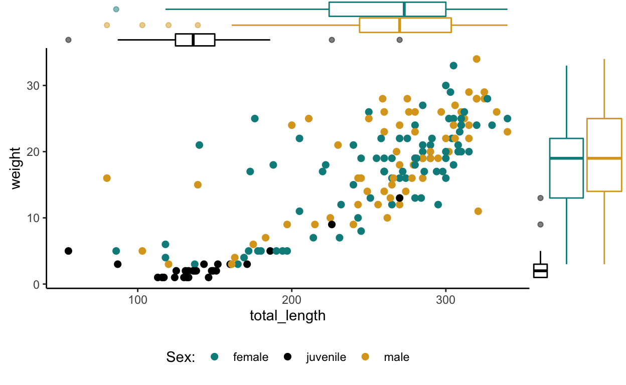
hide

j <- ggplot(data = whiptails, aes(x = total_length, y = weight)) +
  geom_point(aes(color = sex), size = 2) + 
  scale_color_manual(values = c("cyan4", "black", "goldenrod"),
                     name = "Sex:",
                     labels = c("female", "juvenile", "male")) +
   theme_classic() +
  theme(legend.position = "bottom")

ggMarginal(j, type = "boxplot", groupColour = T)

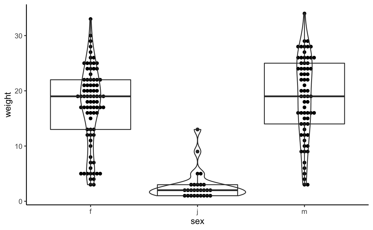
hide

ggplot(whiptails, aes(x = sex, y = weight)) +
  geom_beeswarm() +
  geom_violin(fill = NA) +
  geom_boxplot(fill = NA) +
  theme_classic()

hide

lizard_counts <- liz %>% 
  mutate(date = mdy(date)) %>% 
  mutate(year = year(date)) %>% 
  count(year, common_name) %>% 
  rename(count = n)

hide

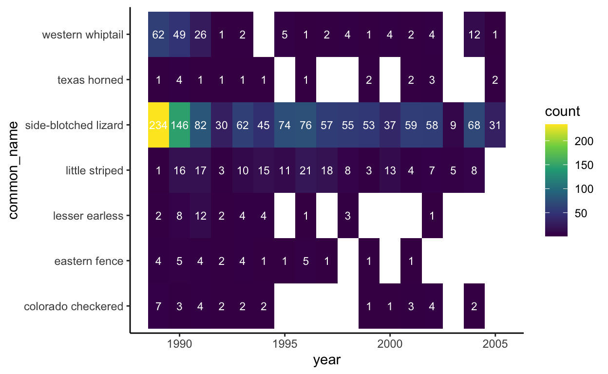
ggplot(data = lizard_counts, aes(x = year, y = common_name)) +
  theme_classic() +
  geom_tile(aes(fill = count)) +
  geom_text(aes(label = count), color = "white", size = 3) +
  scale_fill_gradientn(colors = c("navy", "red", "orange")) + 
  scale_fill_viridis_c()

hide

jornada_veg <- read_sf(here("spatial_vegetation", "doc.kml")) %>% 
  select(Name) %>% 
  clean_names()

ggplot(data = jornada_veg) +
  geom_sf(aes(fill = name), color = NA) +
  scale_fill_viridis_d() +
  theme_minimal() +
  labs(x =  "Longitude",
       y = "Latitude",
       fill = "Dominant vegetation:")