Read & Clean Data
Read in the four datasets containing the chemistry of stream water from the Luquillo Mountains using read_csv(). Tidied data using clean_names() and changed the dates to ISO 8601 format using lubridate.
Q1 <- read_csv(here("/courses", "EDS214", "eco-warriors", "data", "QuebradaCuenca1-Bisley.csv" ),
               na = "-9999") %>%
  clean_names() %>%
  mutate(sample_date = mdy(sample_date))


Q2 <- read_csv(here("/courses", "EDS214", "eco-warriors", "data", "QuebradaCuenca2-Bisley.csv"),
               na = "-9999") %>%
  clean_names() %>%
  mutate(sample_date = mdy_hm(sample_date))


Q3 <- read_csv(here("/courses", "EDS214", "eco-warriors", "data", "QuebradaCuenca3-Bisley.csv"),
               na = "-9999") %>%
  clean_names() %>%
  mutate(sample_date = mdy(sample_date))


RPM <- read_csv(here("/courses", "EDS214", "eco-warriors", "data", "RioMameyesPuenteRoto.csv"),
                na = "-9999") %>%
  clean_names() %>%
  mutate(sample_date = mdy(sample_date))
Data Wrangling
Selecting Variables of Interest
Selected the relevant variables to be used in our graph in order to simplify the dataset.
Q1.1 <- Q1 %>%
  select(sample_id, sample_date, k, no3)


Q2.1 <- Q2 %>%
  select(sample_id, sample_date, k, no3)


Q3.1 <- Q3 %>%
  select(sample_id, sample_date, k, no3)


RPM.1 <- RPM %>%
  select(sample_id, sample_date, k, no3)
Isolating the Year using lubridate
Binding the datasets
Used rbind() to bind the datasets. We used rbind() because it stacked the datasets without adding extra columns. full_join() was considered, as it would have performed the same function
combined_sites <- rbind(Q1.1, Q2.1, Q3.1, RPM.1)
Summarize Data
Grouping Data
Grouped and summarized the data by year, taking the mean Potassium and Nitrate measurements, using group_by() % summarize()
Editing Data
Changed the names of the elements in the data frame and reordered them so that the levels match the figure.
combined_sites_summarize$sample_id <- str_replace(combined_sites_summarize$sample_id,
                                                  "MPR",
                                                  "Puente Roto Mameyes")
combined_sites_summarize$sample_id <- str_replace(combined_sites_summarize$sample_id,
                                                  "Q1",
                                                  "Quebrada uno-Bisley")
combined_sites_summarize$sample_id <- str_replace(combined_sites_summarize$sample_id,
                                                  "Q2",
                                                  "Quebrada dos-Bisley")
combined_sites_summarize$sample_id <- str_replace(combined_sites_summarize$sample_id,
                                                  "Q3",
                                                  "Quebrada tres-Bisley")
combined_sites_summarize$sample_id <- factor(combined_sites_summarize$sample_id,
                                              levels = c("Quebrada dos-Bisley",
                                                        "Quebrada uno-Bisley",
                                                        "Quebrada tres-Bisley",
                                                        "Puente Roto Mameyes"))
Data Visualization
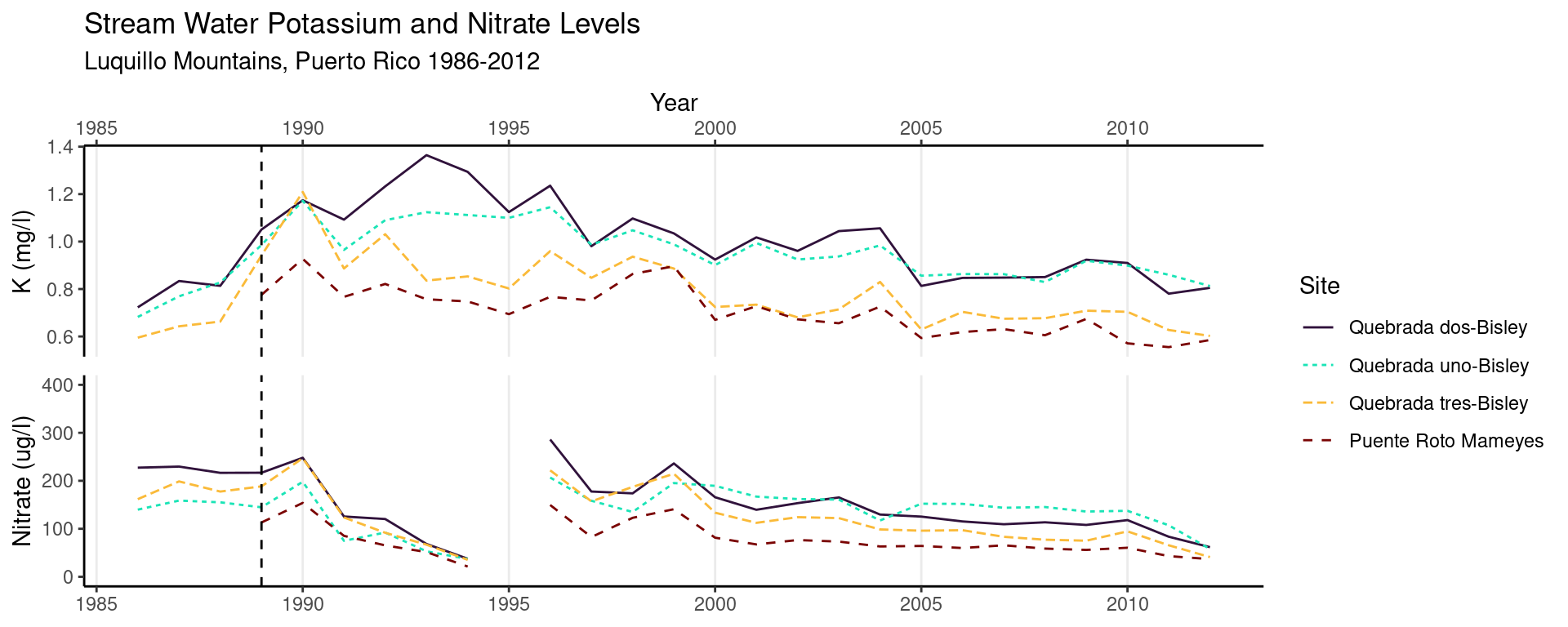
Created two line graphs using ggplot() for annual site means of Potassium and Nitrate. The data was sorted by site_id, displaying the varying levels for each site in the Luquillo Mountains. We then performed data visualization to customize our graph and make it reader friendly. Used patchwork library to combine the graphs.
# Potassium graph
k_graph <- ggplot(data = combined_sites_summarize, aes(x = sample_year, y = mean_k)) +
  geom_line(aes(color = sample_id, linetype = sample_id)) +
  geom_vline(xintercept = (1989),
             linetype = "dashed") +
  labs(x = "Year",
       y = "K (mg/l)",
       title = "Stream Water Potassium and Nitrate Levels",
       subtitle = "Luquillo Mountains, Puerto Rico 1986-2012",
       color = "Site",
       linetype = "Site") +
  theme_classic() +
  scale_x_continuous(position = "top") +
  scale_color_viridis_d(option = "H") +
  theme(plot.margin = unit(c(0, 0, 0.0001, 0), "inches"),
        panel.grid.major.x = element_line(),
        legend.position = "none")


# Nitrate graph
no3_graph <- ggplot(data = combined_sites_summarize, aes(x = sample_year, y = mean_no3)) +
  geom_line(aes(color = sample_id, linetype = sample_id)) +
  geom_vline(xintercept = (1989),
             linetype = "dashed") +
  labs(x = element_blank(),
       y = "Nitrate (ug/l)",
       title = element_blank(),
       color = "Site",
       linetype = "Site") +
  theme_classic() +
  scale_color_viridis_d(option = "H") +
  theme(legend.position = "none",
        axis.title.x.bottom = element_blank(),
        axis.line.x.top = element_line(),
        axis.ticks.x.top = element_line(),
        plot.margin = unit(c(0.0001, 0, 0, 0), "inches"),
        panel.grid.major.x = element_line()) +
  scale_y_continuous(limits = c(0,400))


# Make combined graph with a single centered legend
combined <- k_graph / no3_graph & theme(legend.position = "right")
combined + plot_layout(guides = "collect")

Analysis
Stream water samples were collected weekly from eight sites within the Luquillo Mountains in Puerto Rico from 1986 - 2012. This data reveals how stream chemistry responds to a major hurricane event. The water’s chemical composition from four selected sites graphed over time reveals dramatic fluctuations in potassium and nitrate levels after Hurricane Hugo in 1989.
Potassium (measured in mg/l) at all sites increased steadily from 1986 to 1989, and spiked dramatically for two years following Hurricane Hugo in 1989. This is likely due to increased quantities of plant debris in the stream systems as a result of the hurricane. The sampling site at Quebrada dos-Bisley saw the most extreme increase in potassium levels, peaking in 1993. The sampling site at Puente Roto Mameyes maintained the the most stable potassium levels during this influx period. In the years following 1993, we see a gradual decline at all sites over time with minor fluctuations from 2000 - 2005.
Nitrate levels (measured in ug/l) at all sites remained relatively stable from 1986 to 1990, but increased dramatically following Hurricane Hugo in 1989. This is likely due to the increased plant debris that caused a similar increase in potassium levels. Data was unavailable in the years immediately following 1993, but beginning in 1996 we see the nitrate levels are steading decreasing through 2010.
Citation
Link to Github Repository: https://github.com/julietcohen/EDS-214-eco-warriors
McDowell, W. 2021. Chemistry of stream water from the Luquillo Mountains ver 4923052. Environmental Data Initiative. https://doi.org/10.6073/pasta/ddb4d61aea2fb18b77540e9b0c424684 (Accessed 2021-08-25)