# I found the SST and Chloro data through an old co-worker who was working with the Aqua Modis satelite. # I found the buoy data by scrolling through the NOAA site. See README.md for more info about data.

#Read in Aqua Modis Data
require("rerddap")


#SST for each Buoy
E_sst <- griddap('erdMWsstd8day_LonPM180', # 8 day composite SST E_buoy
 time = c('2020-01-01T12:00:00Z','2021-01-01T12:00:00Z'), # Full year time period 2020
 latitude = c(34.0, 34.5), #grid surrounding buoy
 longitude = c(-119.5, -120), #grid surrounding buoy
 fmt = "csv")  %>%
  add_column(location = "east") #add ID column

W_sst <- griddap('erdMWsstd8day_LonPM180', # 8 day composite SST W_buoy
 time = c('2020-01-01T12:00:00Z','2021-01-01T12:00:00Z'), # Full year time period 2020
 latitude = c(34.0, 34.5), #grid surrounding buoy
 longitude = c(-120, -120.5), #grid surrounding buoy
 fmt = "csv") %>%
  add_column(location = "west") #add ID column

SM_sst <- griddap('erdMWsstd8day_LonPM180', # 8 day composite SST SM_buoy
 time = c('2020-01-01T12:00:00Z','2021-01-01T12:00:00Z'), # Full year time period 2020
 latitude = c(33.5, 34.0), #grid surrounding buoy
 longitude = c(-118.75, -119.25), #grid surrounding buoy
 fmt = "csv") %>%
  add_column(location = "SM") #add ID column

sst <- rbind(E_sst, W_sst, SM_sst) #bind data


#Chloro for each Buoy
E_chloro <- griddap('erdMWchla8day_LonPM180',  # 8 day composite Chlorophyll E_buoy
  time = c('2020-01-01T12:00:00Z','2021-01-01T12:00:00Z'), # Full year time period 2020
  latitude = c(34.0, 34.5), #grid surrounding buoy
  longitude = c(-119.5, -120), #grid surrounding buoy
  fmt = "csv") %>%
  add_column(location = "east") #add location term

W_chloro <- griddap('erdMWchla8day_LonPM180', # 8 day composite Chlorophyll E_buoy
  time = c('2020-01-01T12:00:00Z','2021-01-01T12:00:00Z'), # Full year time period 2020
  latitude = c(34.0, 34.5), #grid surrounding buoy
  longitude = c(-120, -120.5), #grid surrounding buoy
  fmt = "csv") %>%
  add_column(location = "west") #add location term

SM_chloro <- griddap('erdMWchla8day_LonPM180', # 8 day composite Chlorophyll SM_buoy
  time = c('2020-01-01T12:00:00Z','2021-01-01T12:00:00Z'), # Full year time period 2020
  latitude = c(33.5, 34.0), #grid surrounding buoy
  longitude = c(-118.75, -119.25), #grid surrounding buoy
  fmt = "csv")%>%
  add_column(location = "SM") #add location term

chloro <- rbind(E_chloro, W_chloro, SM_chloro) #Bind data


#Wind data for each buoy and data cleaning
tab_E <- read.table(here("_posts", "2021-10-31-combining-data", "data","east_wind.txt"), comment="", header=TRUE) #convert .txt file to .csv
write.csv(tab_E, "east_wind.csv", row.names=F, quote=F)

E_wind <- read.csv(here("_posts", "2021-10-31-combining-data","east_wind.csv")) %>% # read in .csv, select coloumns and rename
  add_column(location = "east") %>%
  dplyr::select(c("X.YY", "MM", "DD", "WSPD", "location"))  %>%
  rename(year = X.YY,
         month = MM,
         day = DD)
E_wind <- E_wind[-c(1),]


tab_W <- read.table(here("_posts", "2021-10-31-combining-data","data","west_wind.txt"), comment="", header=TRUE) #convert .txt file to .csv
write.csv(tab_W, "west_wind.csv", row.names=F, quote=F)

W_wind <- read.csv(here("_posts", "2021-10-31-combining-data","west_wind.csv"))%>% # read in .csv, select coloumns and rename
  add_column(location = "west") %>%
  dplyr::select(c("X.YY", "MM", "DD", "WSPD", "location"))  %>%
  rename(year = X.YY,
         month = MM,
         day = DD)
W_wind <- W_wind[-c(1),]


tab_SM <- read.table(here("_posts", "2021-10-31-combining-data","data","SM_wind.txt"), comment="", header=TRUE) #convert .txt file to .csv
write.csv(tab_SM, "SM_wind.csv", row.names=F, quote=F)

SM_wind <- read.csv(here("_posts", "2021-10-31-combining-data","SM_wind.csv"))%>% # read in .csv, select coloumns and rename
  add_column(location = "SM") %>%
  dplyr::select(c("X.YY", "MM", "DD", "WSPD", "location"))  %>%
  rename(year = X.YY,
         month = MM,
         day = DD)
SM_wind <- SM_wind[-c(1),]

wind <- rbind(E_wind, W_wind, SM_wind) #bind data
#clean date format and summarize with daily means for wind

wind <- wind %>%
  unite("date", year:month:day, sep = "-") %>%
  mutate(date = ymd(date, tz = NULL)) %>%
  mutate(WSPD = as.numeric(WSPD))

# see the data join chunk for na.rm explanation in code comment

wind_avg <- wind %>%
  group_by(location, date) %>%
  summarize(mean_wind = mean(WSPD, na.rm = T))
#Clean sst Data and summarize by daily means
final_sst <- sst_clean %>%
  filter(sst > 0) %>% #remove NAs
  mutate(sst = (sst * (9/5) + 32 )) %>% #convert to F
  mutate(sst = (sst - 3)) #accounting for SST Satelite error through anecdotal and buoy comparison.

# see the data join chunk for na.rm explanation in code comment

final_sst_avg <- final_sst %>%
  group_by(location, date) %>%
  summarize(mean_sst = mean(sst, na.rm = T))
#clean chloro data
# see the data join chunk for na.rm explanation in code comment

chloro_clean <- chloro %>%
  mutate(date = ymd_hms(time, tz = "UTC")) %>%
  mutate(ymd_date = ymd(date, tz = NULL)) %>%
  mutate(date = ymd_date) %>%
  dplyr::select(c("latitude", "longitude", "chlorophyll", "location", "date"))

final_chloro_avg <- chloro_clean %>%
  group_by(location, date) %>%
  summarize(mean_chloro = mean(chlorophyll, na.rm = T))
#combine daily wind and sst and chloro means
# we changed left join to inner join in order to not include any rows that lack values for ANY of the 3 variables. We do not want any NA values in one col and have data in another col, because when we map everything together that data would be represented as if there was a zero value for tyhe variable that had NA. This change reduced the amount of rows by a couple hundred, This was primarily for the SST and Cholor data which had NA's but the wind data did not initially have NA's.

wind_sst <- inner_join(wind_avg, final_sst_avg, by = c("date", "location"))

chloro_wind_sst <- inner_join(wind_sst, final_chloro_avg, by = c("date", "location"))
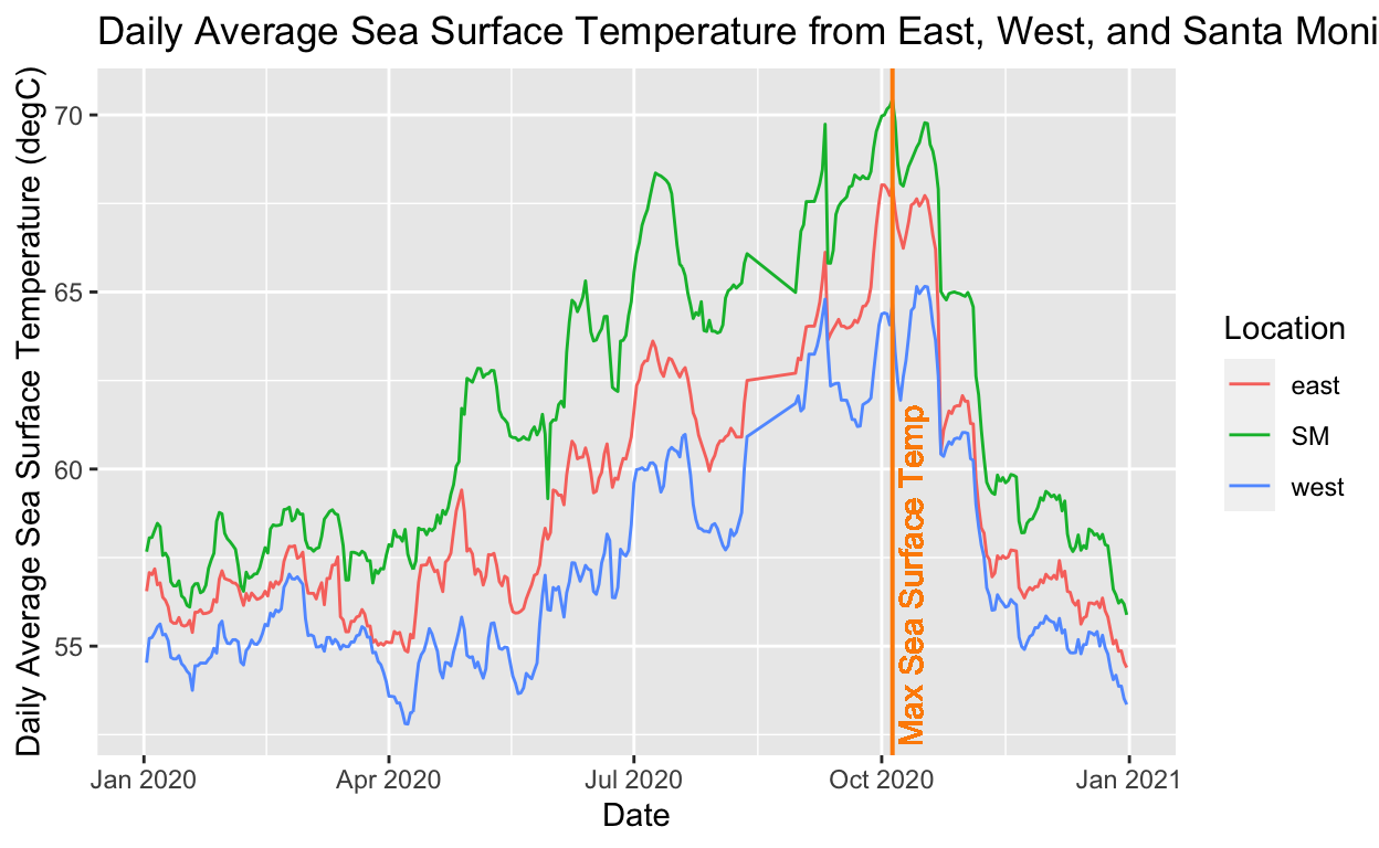
#Daily Average Sea Surface Temperature from East, West, and Santa Monica Buoys

# calculate the average max SST value

max_sst_value <- max(chloro_wind_sst$mean_sst)
max_sst_value
[1] 70.43606# filter the dataset for this value, so you can determine the date when the max value occurred, so you know where on the x-axis you should plot the vline to represent the max value
data_max_sst <- chloro_wind_sst %>%
filter(mean_sst == max_sst_value)
# plot the graph with the vline at the max value
ggplot(data = chloro_wind_sst, aes(x = date, y = mean_sst, color = location)) +
geom_line() +
geom_vline(xintercept = data_max_sst$date,
size = 0.7,
color = "darkorange") +
geom_text(aes(x = data_max_sst$date,
label = "Max Sea Surface Temp",
y = 57),
angle = 90,
vjust = 1.3,
text = element_text(size = 14),
color = "darkorange") +
labs(x = "Date",
y = "Daily Average Sea Surface Temperature (degC)",
title = "Daily Average Sea Surface Temperature from East, West, and Santa Monica Buoys",
color = "Location")
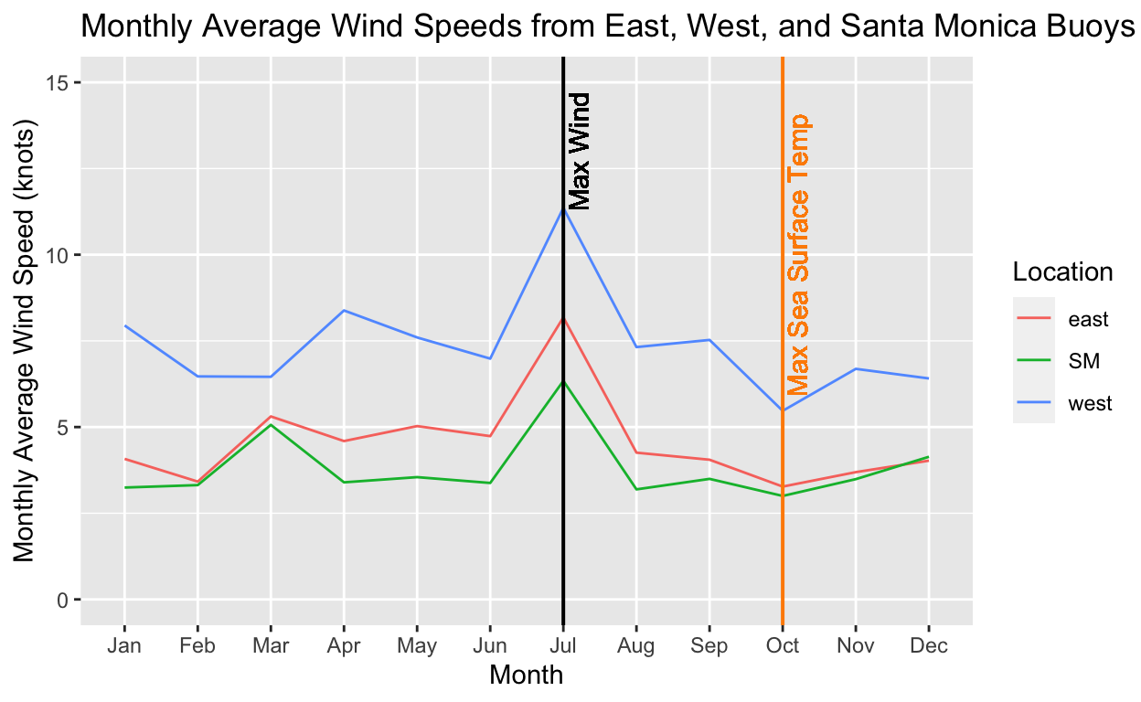
#Monthly Average Wind from East, West, and Santa Monica Buoys

month_mean <- chloro_wind_sst %>%
  dplyr::select(location, date, mean_wind) %>%
  mutate(month = month(date, label = TRUE)) %>%
  mutate(month = as.numeric(month)) %>%
  group_by(location, month) %>%
  summarize(mean_wind = mean(mean_wind, na.rm = T))

# find the max wind
max_wind_value = max(month_mean$mean_wind)
max_wind_value
[1] 11.35845data_max_wind <- month_mean %>%
filter(mean_wind == max_wind_value)
# plot it with the vertical line
ggplot(data = month_mean, aes(x = month, y = mean_wind, color = location)) +
geom_line() +
geom_vline(xintercept = 7,
size = 0.7,
color = "black") +
geom_text(aes(x = 7,
label = "Max Wind",
y = 13),
angle = 90,
vjust = 1.3,
text = element_text(size = 14),
color = "black") +
geom_vline(xintercept = 10,
size = 0.7,
color = "darkorange") +
geom_text(aes(x = 10,
label = "Max Sea Surface Temp",
y = 10),
angle = 90,
vjust = 1.3,
text = element_text(size = 14),
color = "darkorange") +
labs(x = "Month",
y = "Monthly Average Wind Speed (knots)",
title = "Monthly Average Wind Speeds from East, West, and Santa Monica Buoys",
color = "Location") +
ylim(0,15) +
scale_x_discrete(limits=month.abb)
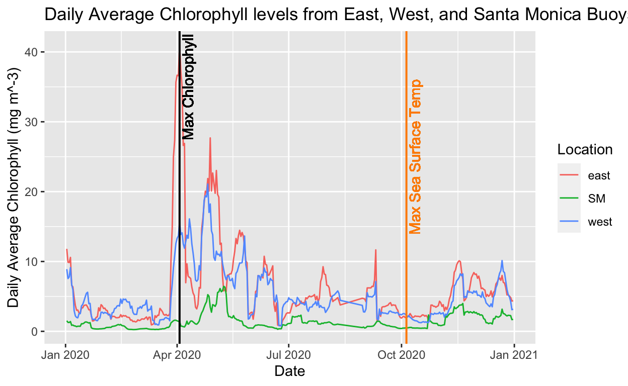
#Daily Average Chorophyll from East, West, and Santa Monica Buoys

# find the max chloro value
max_chloro <- max(chloro_wind_sst$mean_chloro)
max_chloro
[1] 40.94858# find the date for the max chloro value
data_max_chloro <- chloro_wind_sst %>%
filter(mean_chloro == max_chloro)
# plot it with the vertical line on the date of the max chloro value
ggplot(data = chloro_wind_sst, aes(x = date, y = mean_chloro, color = location)) +
geom_line() +
geom_vline(xintercept = data_max_chloro$date,
size = 0.7,
color = "black") +
geom_text(aes(x = data_max_chloro$date,
label = "Max Chlorophyll",
y = 35),
angle = 90,
vjust = 1.3,
text = element_text(size = 14),
color = "black") +
geom_vline(xintercept = data_max_sst$date,
size = 0.7,
color = "darkorange") +
geom_text(aes(x = data_max_sst$date,
label = "Max Sea Surface Temp",
y = 25),
angle = 90,
vjust = 1.3,
text = element_text(size = 14),
color = "darkorange") +
labs(x = "Date",
y = "Daily Average Chlorophyll (mg m^-3)",
title = "Daily Average Chlorophyll levels from East, West, and Santa Monica Buoys",
color = "Location")
Distill is a publication format for scientific and technical writing, native to the web.
Learn more about using Distill at https://rstudio.github.io/distill.