Impact of the February Storm on Power in Huston, TX

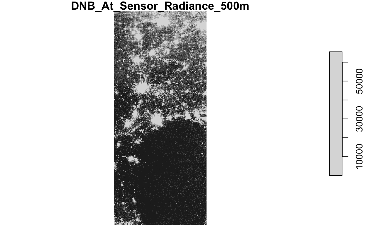
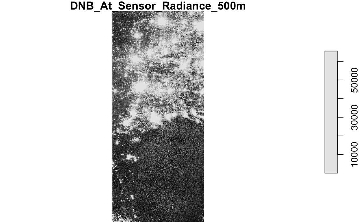
The extreme weather event seen in Houston, TX in February 2021 caused major blackouts due to a power grid failure. Using satellite images, the extent of the blackout can be measured by comparing the night lights before and after the storm.

library(sf)
library(tidyverse)
library(stars)
library(rgdal)
library(stringr)
library(raster)
library(dplyr)
library(patchwork)
library(ggsn)
library(rosm)
library(tmap)
library(here)
library(rnaturalearth)

Function to load the DNB dataset from VNP46A1 granules

read_dnb <- function(file_name) {
  dataset_name <- "//HDFEOS/GRIDS/VNP_Grid_DNB/Data_Fields/DNB_At_Sensor_Radiance_500m"

  h_string <- gdal_metadata(file_name)[199]
  v_string <- gdal_metadata(file_name)[219]
  
  tile_h <- as.integer(str_split(h_string, "=", simplify = TRUE)[[2]])
  tile_v <- as.integer(str_split(v_string, "=", simplify = TRUE)[[2]])

  west <- (10 * tile_h) - 180
  north <- 90 - (10 * tile_v)
  east <- west + 10
  south <- north - 10

  delta <- 10 / 2400

  dnb <- read_stars(file_name, sub = dataset_name)

  st_crs(dnb) <- st_crs(4326)
  st_dimensions(dnb)$x$delta <- delta
  st_dimensions(dnb)$x$offset <- west
  st_dimensions(dnb)$y$delta <- -delta
  st_dimensions(dnb)$y$offset <- north
  
  return(dnb)
}

Add data to dnb function

feb07_5<- "data/VNP46A1.A2021038.h08v05.001.2021039064328.h5"
dnb07_5<- read_dnb(file_name = feb07_5)

//HDFEOS/GRIDS/VNP_Grid_DNB/Data_Fields/DNB_At_Sensor_Radiance_500m,

feb07_6<- "data/VNP46A1.A2021038.h08v06.001.2021039064329.h5"
dnb07_6<- read_dnb(file_name = feb07_6)

//HDFEOS/GRIDS/VNP_Grid_DNB/Data_Fields/DNB_At_Sensor_Radiance_500m,

feb16_5<- "data/VNP46A1.A2021047.h08v05.001.2021048091106.h5"
dnb16_5<- read_dnb(file_name = feb16_5)

//HDFEOS/GRIDS/VNP_Grid_DNB/Data_Fields/DNB_At_Sensor_Radiance_500m,

feb16_6<- "data/VNP46A1.A2021047.h08v06.001.2021048091105.h5"
dnb16_6<- read_dnb(file_name = feb16_6)

//HDFEOS/GRIDS/VNP_Grid_DNB/Data_Fields/DNB_At_Sensor_Radiance_500m,

Combine based on date

#feb 07 data
combined07 <- st_mosaic(dnb07_5,dnb07_6)

plot(combined07)

downsample set to c(9,9)

#feb 16 data
combined16 <- st_mosaic(dnb16_5, dnb16_6)

plot(combined16)

downsample set to c(9,9)

rm(dnb07_5,
   dnb07_6,
   dnb16_5,
   dnb16_6) #remove unneeded files

Create a blackout mask

difference <- (combined07 - combined16) > 200

difference[difference == FALSE] <- NA

The data from after the storm was subtracted from that of before the storm to show the difference in night light caused by the power outage.

Vectorize the mask

blackout <- st_as_sf(difference)

Fix broken polygons

blackout_mask <- st_make_valid(blackout)

Crop the map to ROI

poly <- st_polygon(list(rbind(c(-96.5, 29), 
                              c(-96.5, 30.5), 
                              c(-94.5, 30.5), 
                              c(-94.5, 29), 
                              c(-96.5, 29))))

ROI <-st_sfc(poly, crs = 4326) 


cropped <- blackout_mask[ROI, op = st_intersects]



map <- st_transform(cropped, crs = st_crs(3083))

Account for highways

query <- "SELECT * FROM gis_osm_roads_free_1 
WHERE fclass='motorway'"
roads <- ("data/gis_osm_roads_free_1.gpkg")
highways <- st_read(roads, query = query)

Reading query `SELECT * FROM gis_osm_roads_free_1 
WHERE fclass='motorway'' from data source `/Users/JaketheBoss/Documents/Bren/Jake-Eisaguirre.github.io/_posts/2021-11-08-houston-ice-storm/data/gis_osm_roads_free_1.gpkg' 
  using driver `GPKG'
Simple feature collection with 6085 features and 10 fields
Geometry type: LINESTRING
Dimension:     XY
Bounding box:  xmin: -96.50429 ymin: 29.00174 xmax: -94.39619 ymax: 30.50886
Geodetic CRS:  WGS 84

highways <- st_transform(highways, crs = st_crs(3083))

hwy_buffer200m <- st_buffer(highways, dist = 200)
hwy_dissolve <- st_union(hwy_buffer200m)

Buildings Data

query_1 <- "SELECT * FROM gis_osm_buildings_a_free_1 
WHERE (type IS NULL AND name IS NULL) OR 
type in ('residential', 'apartments', 'house', 'static_caravan', 'detached')"
buildings <- "data/gis_osm_buildings_a_free_1.gpkg"
houses <- st_read(buildings, query = query_1)

Reading query `SELECT * FROM gis_osm_buildings_a_free_1 
WHERE (type IS NULL AND name IS NULL) OR 
type in ('residential', 'apartments', 'house', 'static_caravan', 'detached')' from data source `/Users/JaketheBoss/Documents/Bren/Jake-Eisaguirre.github.io/_posts/2021-11-08-houston-ice-storm/data/gis_osm_buildings_a_free_1.gpkg' 
  using driver `GPKG'
Simple feature collection with 475941 features and 5 fields
Geometry type: MULTIPOLYGON
Dimension:     XY
Bounding box:  xmin: -96.50055 ymin: 29.00344 xmax: -94.53285 ymax: 30.50393
Geodetic CRS:  WGS 84

houses <- st_transform(houses, crs = st_crs(3083))

Cencus Tract Data

cencus <- "data/ACS_2019_5YR_TRACT_48_TEXAS.gdb"

acs_geoms <- st_read(cencus,layer = "ACS_2019_5YR_TRACT_48_TEXAS")

Reading layer `ACS_2019_5YR_TRACT_48_TEXAS' from data source 
  `/Users/JaketheBoss/Documents/Bren/Jake-Eisaguirre.github.io/_posts/2021-11-08-houston-ice-storm/data/ACS_2019_5YR_TRACT_48_TEXAS.gdb' 
  using driver `OpenFileGDB'
Simple feature collection with 5265 features and 15 fields
Geometry type: MULTIPOLYGON
Dimension:     XY
Bounding box:  xmin: -106.6456 ymin: 25.83716 xmax: -93.50804 ymax: 36.5007
Geodetic CRS:  NAD83

acs_income <- st_read(cencus,layer = "X19_INCOME")

Reading layer `X19_INCOME' from data source 
  `/Users/JaketheBoss/Documents/Bren/Jake-Eisaguirre.github.io/_posts/2021-11-08-houston-ice-storm/data/ACS_2019_5YR_TRACT_48_TEXAS.gdb' 
  using driver `OpenFileGDB'

median_income <- acs_income[c("GEOID", "B19013e1")]

median_income <- median_income %>% 
  rename(median_income = B19013e1)

Merge data sets

remove_highways <- st_difference(map, hwy_dissolve)

tot_num_of_houses_no_power <- houses[remove_highways, op = st_intersects]  

nrow(tot_num_of_houses_no_power)

[1] 157411

texas_map <- ne_countries(country = 'united states of america', 
                         scale = 'large', returnclass = 'sf')

query_1 = "
  SELECT fclass, geom
  FROM gis_osm_roads_free_1
  WHERE fclass in ('motorway', 'motorway_link', 'primary', 'primary_link')"
highways2 = st_read("data/gis_osm_roads_free_1.gpkg", query = query)

Reading query `SELECT * FROM gis_osm_roads_free_1 
WHERE fclass='motorway'' from data source `/Users/JaketheBoss/Documents/Bren/Jake-Eisaguirre.github.io/_posts/2021-11-08-houston-ice-storm/data/gis_osm_roads_free_1.gpkg' 
  using driver `GPKG'
Simple feature collection with 6085 features and 10 fields
Geometry type: LINESTRING
Dimension:     XY
Bounding box:  xmin: -96.50429 ymin: 29.00174 xmax: -94.39619 ymax: 30.50886
Geodetic CRS:  WGS 84

Houston_map <- ggplot() +
  geom_sf(data = texas_map, fill = NA, color = 'black') +
  geom_sf(data = houses,color = "grey") +
  geom_sf(data = tot_num_of_houses_no_power, color = 'black')+
  geom_sf(data = highways2, color = "grey20") +
  theme_minimal() +
  ylab("Latitude") +
  xlab("Longitude") +
  ggtitle("Impact of 2021 Storm on Residential Houses in Houston") +
  theme(panel.border = element_rect(colour = "black", fill=NA, size=1)) + 
  coord_sf(xlim = c(-94.5, -96.5), ylim = c(29, 30.5), expand = F) +
  north(x.min = -94.5, x.max = -96.5, y.min = 29, y.max = 30.5, scale = 0.15, location = "topright") +
  scalebar(x.min = -94.5, x.max = -96.5, y.min = 29, y.max = 30.5, dist = 25, dist_unit = "km", 
           transform = T, 
           st.bottom = F,
           location = "bottomleft",
           anchor = c(x = -95.2, y = 29.01))
Houston_map

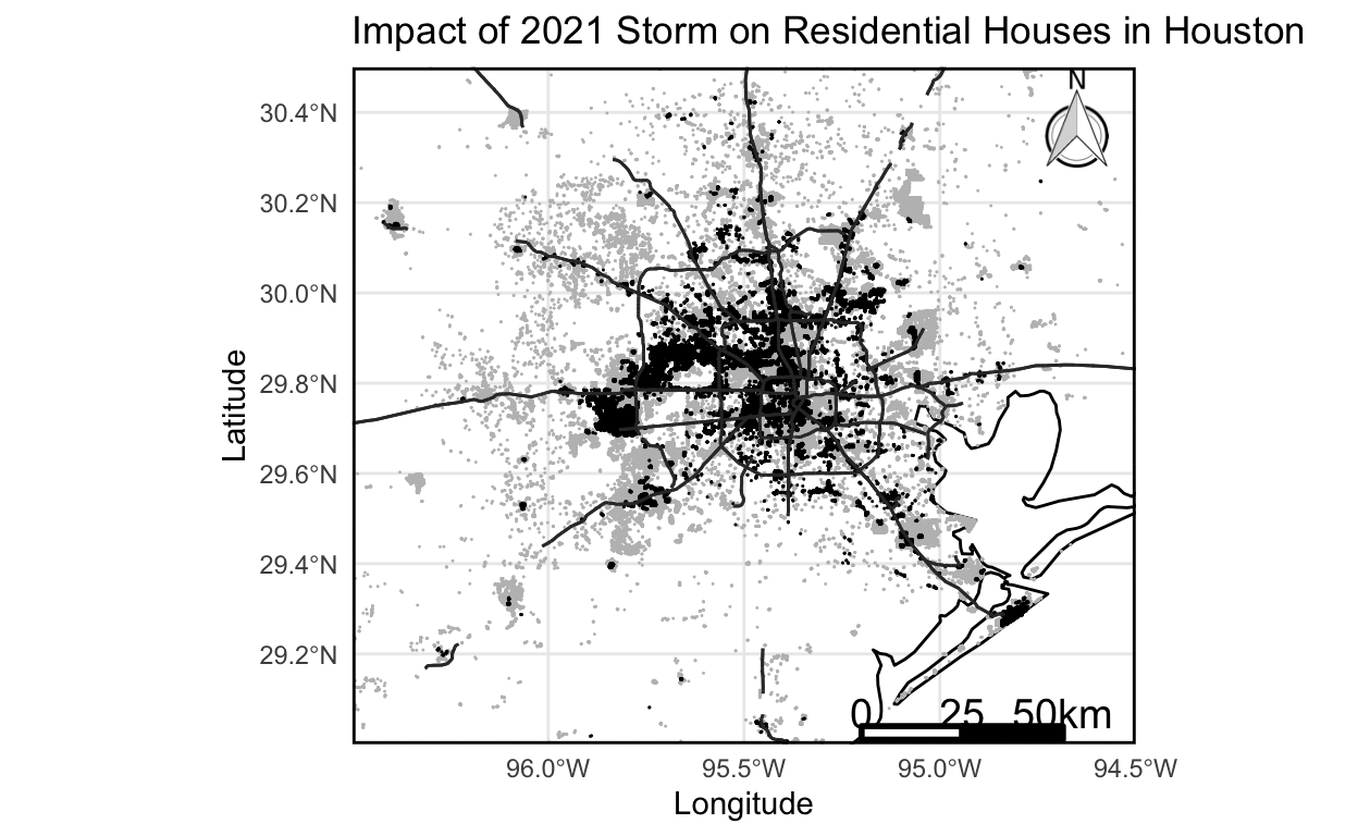
Grey layer is the total number of residential houses in Houston and the black layer is the total number of residential houses that lost power from the 2021 ice storm. Dark gray lines are major road ways and dark black lines are Texas coastline.

Due to the light pollution caused by highways, highways were removed from the dataset to not be included in the change of light. Comparing the night lights of February 16, 2021 to February 7, 2021, it appears that 157,411 houses were impacted by the power grid failure.

Socioeconomic Impact

socio_eco <- left_join(acs_geoms, median_income, by = c("GEOID_Data" = "GEOID"))

Residential_income <- ggplot(data = socio_eco) +
  geom_histogram(aes(x = median_income)) +
  theme_classic() +
  geom_vline(xintercept = 55771,
             col = 'red',
             lwd = 1)+
  annotate("text",
           x = 150000,
           y = 350,
           label = paste("Median = $55,771.00"),
           col = 'red')+
  geom_vline(xintercept = 64120.33,
             col = 'blue',
             lwd = 1)+
  annotate("text",
           x = 150000,
           y = 400,
           label = paste("Mean = $64,120.33"),
           col = 'blue') +
  ggtitle("Median Income of Residential Buildings in Houston")#all of houston

Residential_income

socio_eco <- st_transform(socio_eco, crs = st_crs(3083))
lost_power_income <- socio_eco[tot_num_of_houses_no_power, op = st_intersects]


Blackout_income <- ggplot(data = lost_power_income) +
  geom_histogram(aes(x = median_income)) +
  theme_classic() +
  geom_vline(xintercept = 60414.5,
             col = 'red',
             lwd = 1)+
  annotate("text",
           x = 150000,
           y = 50,
           label = paste("Median = $60,414.50"),
           col = 'red')+
  geom_vline(xintercept = 71244.88,
             col = 'blue',
             lwd = 1)+
  annotate("text",
           x = 150000,
           y = 75,
           label = paste("Mean = $71,244.88"),
           col = 'blue') +
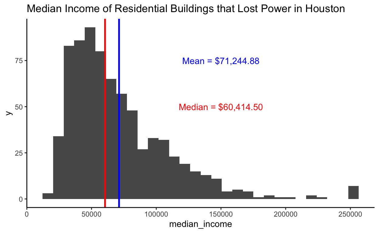
  ggtitle("Median Income of Residential Buildings that Lost Power in Houston")#ice storm

Blackout_income

na_median <- na.omit(median_income)
median(na_median$median_income)

[1] 55771

mean(na_median$median_income)

[1] 64130.33

na_median_power <- na.omit(lost_power_income)
median(na_median_power$median_income)

[1] 60414.5

mean(na_median_power$median_income)

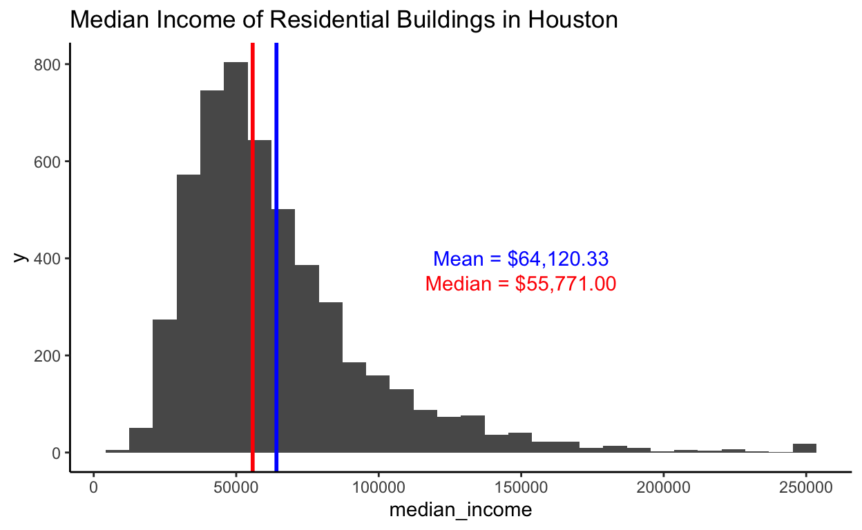
[1] 71244.88

Median income of all of Houston = $55,771.00 Mean income of all of Houston = $64,120.33 Median income of those that lost power in Houston = $60,414.50 Mean income of those that lost power in Houston = $71,244.88

Median income is not a factor in determining if a house will be affected by loss of power. There was a slightly higher median income with the houses that lost power.

Houston Ice Storm