Introduction
The Northern Channel Islands are situated in the Southern California Bight 22 miles from Santa Barbara California. They are known to be a biodiversity hotpot due to unique environmental factors driving local ecological processes (Santa Barbara ChannelKeeper). In 2003 the state of California, along with NOAA, created 10 Marine protected areas (MPAs) and designated the Channel islands a marine sanctuary. The creation of no-take MPAs allowed for a release of commercial and recreational fishing pressures (National Park Service). Just Prior to the creation of the MPAs, the Partnership for Interdisciplinary Studies of Coastal Oceans (PISCO), began conducting sub-tidal kelp forest surveys inside a suite of MPAs and reference sites in order to gain a better understanding how the release of fishing pressure might alter ecological interactions.
Northern Channel Islands Map
hide
cha <- read_sf(here("_posts", "2021-11-29-mpasandkelp", "shape", "channel_islands.shp")) %>%
mutate(geometry = st_transform(geometry, "+proj=longlat +ellps=WGS84 +datum=WGS84")) %>%
filter(!NAME=="San Clemente")
ca <- read_sf(here("_posts", "2021-11-29-mpasandkelp","s_11au16", "s_11au16.shp")) %>%
mutate(geometry = st_transform(geometry, "+proj=longlat +ellps=WGS84 +datum=WGS84")) %>%
filter(NAME == "California")
MPA <- read_sf(here("_posts", "2021-11-29-mpasandkelp","ds582", "ds582.shp")) %>%
mutate(geometry = st_transform(geometry, "+proj=longlat +ellps=WGS84 +datum=WGS84")) %>%
filter(OBJECTID %in% c(101:114))
ggplot() +
scale_x_continuous("Longitude", breaks = c(-120.5, -120.25, -120, -119.75, -119.5, -119.25),
expand = c(0,0)) +
scale_y_continuous("Latitude", breaks = c(33.25, 33.5, 33.75, 34, 34.25, 34.5),
expand = c(0,0),
position = "left") +
geom_sf(data = cha, color = "black", fill = "grey60") +
geom_sf(data = ca, color = "black", fill = "grey60") +
theme_classic() +
geom_sf(data = MPA, color = "red", fill = "red", alpha = 0.3, show.legend = T) +
coord_sf(xlim = c(-120.75, -119.0), ylim = c(33.8, 34.75), expand = T) +
geom_text(aes(x = -120.4, y = 34.2), label = "San Miguel" ) +
geom_text(aes(x = -120.12, y = 34.1), label = "Santa Rosa" ) +
geom_text(aes(x = -119.72, y = 34.1), label = "Santa Cruz" ) +
geom_text(aes(x = -119.35, y = 34.1), label = "Anacapa" ) +
geom_point(aes(x = -119.84, y = 34.42), shape = 18, size = 3.3) +
geom_text(aes(x = -119.84, y = 34.48), label = "Bren Hall") +
scalebar(x.min = -120.75, x.max = -119.0, y.min = 33.8, y.max = 34.75,
dist = 15, dist_unit = "km",
transform = TRUE, model = "WGS84", st.bottom = F,
location = "bottomleft",
anchor = c(x = -120.7, y = 33.8), #add scale bar and set location
st.dist = 0.03) +
north(x.min = -120.75, x.max = -119.0, y.min = 33.8, y.max = 34.75,
scale = 0.15, anchor = c(x = -119.05, y = 34.72) ) +
theme(panel.border = element_rect(colour = "black", fill=NA, size=1),
axis.ticks = element_line(size = 0.5, color = "black")) +
scale_colour_manual(name = "Site Status", values = c(MPA = "red")) +
theme(legend.title = element_text(size = 10),
legend.text = element_text(size = 10),
legend.position = c(0.1, 0.60),
plot.caption = element_text(hjust = 0)) +
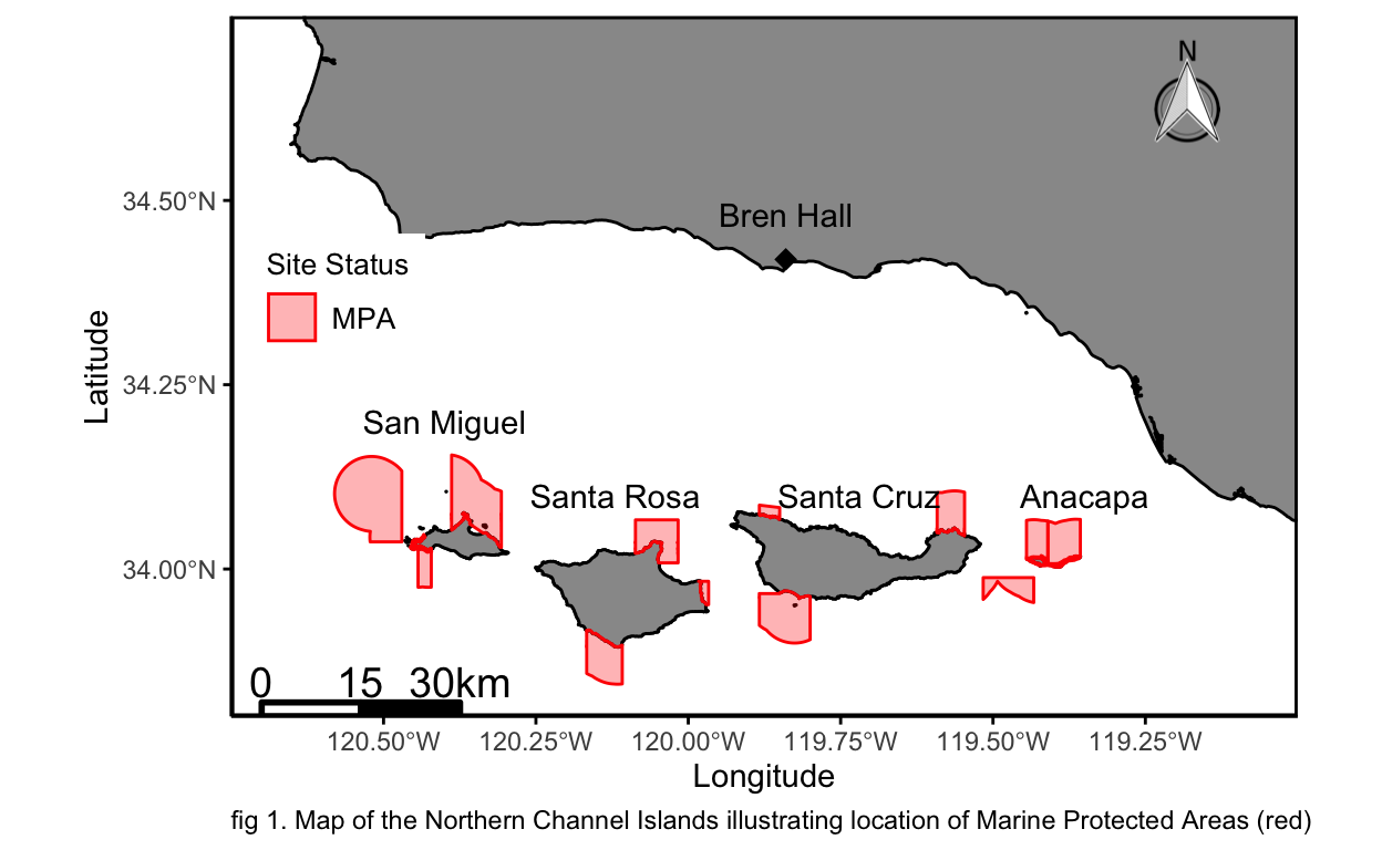
labs(caption = "fig 1. Map of the Northern Channel Islands illustrating location of Marine Protected Areas (red)")
An array work has already been done analyzing the effects of MPA implementation on Kelp Forests (Hamilton & Caselle, 2015, Selden et al. 2017). It is well known that many trophic levels change in abundance whether in an MPA or in a fished area (A Decade of Protection, PISCO). It is also well know that Purple urchins can form “barrens” when densities reach a critical threshold (Ling et al., 2015). There is a tipping point where a phase-shift occurs from a macro-algae dominated system to an urchin barren (Dexter & Scheibling, 2014). The reef will become completely devoid of algae and the dominate space holder will be purple urchins(Ling et al., 2015, Dexter & Scheibling, 2014).
I began conducting sub-tidal surveys for PISCO in 2017 and have developed these questions based on anecdotal evidence. It was always visually evident if we were surveying in an MPA or reference site based on kelp and urchin densities. MPAs visually had more kelp and less urchins while reference sites visually had less kelp and more urchins.
In this study I will test my anecdotal questions with PISCO data. I ask the question; Do MPAs increase kelp densities and what invertebrate species inhibit kelp densities? I also take a simplistic approach and address the question; At what point do MPAs and reference sites kelp densities significantly differ following MPA implementation?
Methods
In order to answer the desired questions I have obtained PISCO data running from 1999 to 2020. I have chosen to look at Anacapa Island, Santa Cruz Island, Santa Rosa Island, and San Miguel Island as those islands are the predominant data source for PISCO N. Channel Island survey sites (fig 1).
Data was collected through annual sub-tidal scuba surveys. 12 benthic transects (30 x 2 x 2 m) are surveyed at each site between June and August to quantify densities of invertebrates and macro-algae. Benthic surveys are stratified into three depth zones (approximately 5-, 10-, and 15-m depth). Giant kelp (Macrocystis pyrifera) (kelp) individuals greater than 1-m in height are counted and stipes are enumerated per individual and later summed at the transect level for analysis. Purple urchins (Strongylocentrotus purpuratus) greater than 2.5 cm in diameter are counted. Sites are either categorized as MPAs or reference sites, each MPA has a paired reference site.
Data was averaged to an annual site mean (n=658, MPA: n=310, Reference: n=348) for purple urchins and kelp stipes (kelp). Understory kelps and red urchins were not included as Giant kelp is the predominant structural species and red urchins are commercially fished.
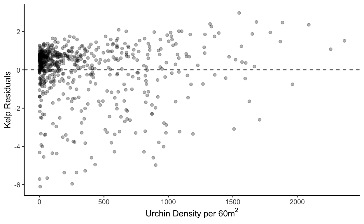
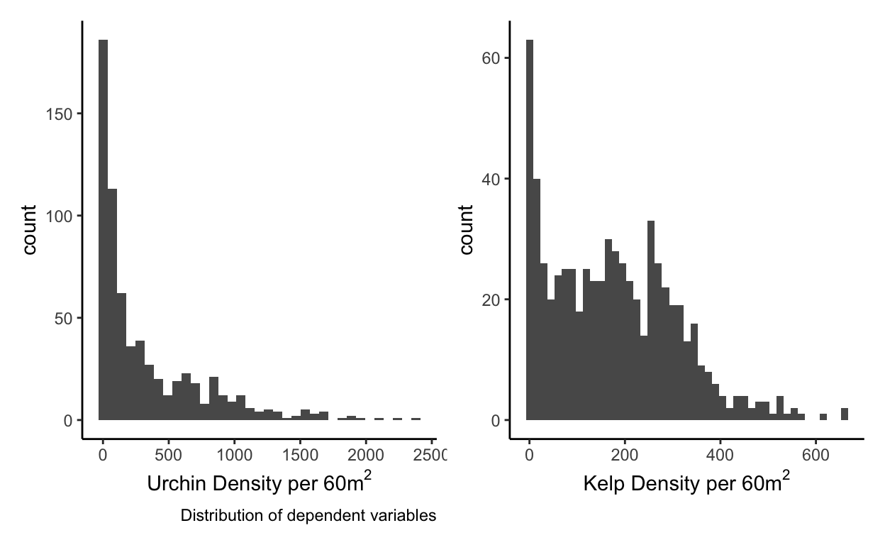
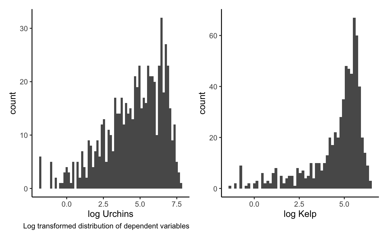
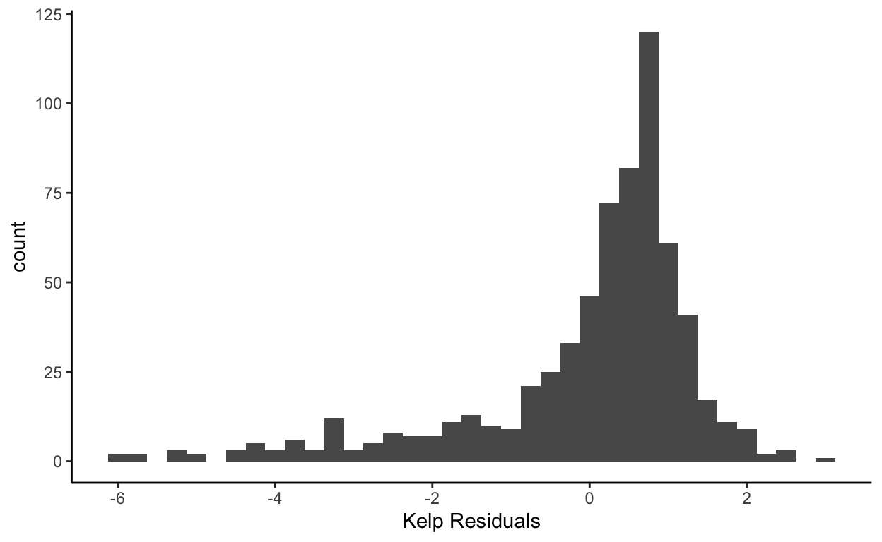
All analysis was conducted in Rstudio and the code repository is linked (see supporting figures). OLS linear models and whelch two sample t tests (\(\alpha\) < 0.05) were conducted based on previous studies understandings of affects purple urchins can have on kelp densities when urchin populations are left unchecked. Response variables were log transformed in order to normalize distribution (see supporting figures). The QQplot is not linear and the residuals show potential heteroscedasticity, model results should guide further research (see supporting figures). All other tests of model fit did show potential for acceptable model choice.
hide
raw_data <- read_csv(here("_posts", "2021-11-29-mpasandkelp", "MLPA_swath_site_means.csv"))


annual_mean <- raw_data %>%
  filter(campus == "UCSB") %>%
  separate(col = site, into = c('island', 'site'), sep = '_') %>%
  filter(island %in% c("ANACAPA", "SCI", "SRI", "SMI")) %>%
  select(c("survey_year", "site", "island", "latitude",
           "longitude", "site_status",
           "den_STRPURAD", "den_MACPYRAD", "den_MACSTIPES")) %>%
  group_by(survey_year, site_status) %>%
  mutate(mean_purp = mean(den_STRPURAD),
         mean_stipe = mean(den_MACSTIPES),
         mean_mac = mean(den_MACPYRAD)) %>%
  mutate(log_urch = log(den_STRPURAD)) %>%
  mutate(log_mac = log(den_MACSTIPES)) %>%
  mutate(log_plant = log(den_MACPYRAD)) %>%
  filter_all(all_vars(!is.infinite(.))) %>%
  ungroup()
Results
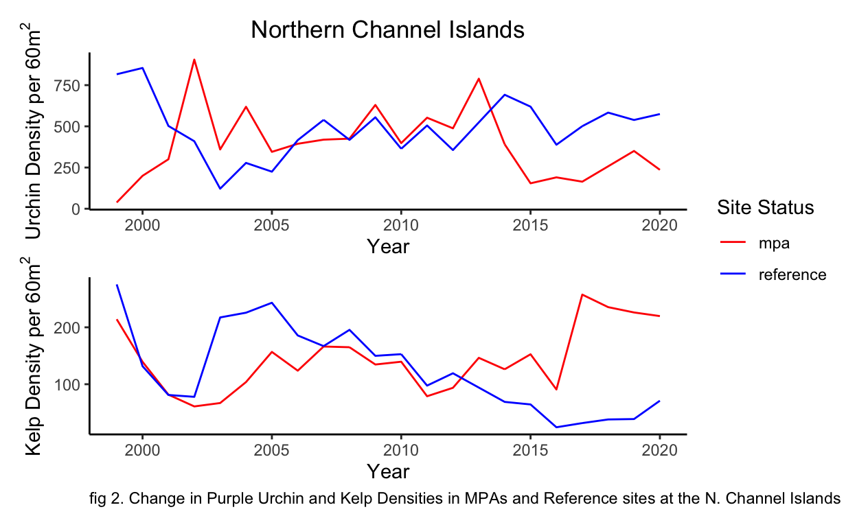
Through initial data visualization, trends can be observed for kelp densities and urchin densities inside MPAs and reference sites (fig 2). It is apparent that urchin densities between MPAs and reference sites fluctuate and follow similar trends until 2014, in which urchin densities inside MPAs show considerably lower densities. A similar trend is observed for kelp densities in which densities fluctuate until 2013 and then began to diverge with higher densities inside the MPAs.
hide
urchins <- ggplot(data = annual_mean) +
  geom_line(aes(x = survey_year, y = mean_purp, color = site_status)) +
  theme_classic() +
  xlab("Year")+
  ylab(expression("Urchin Density per 60m"^2)) +
  labs(color = "Site Status") +
  scale_color_manual(values = c("red", "blue")) +
  labs(title = "Northern Channel Islands") +
  theme(plot.title = element_text(hjust = 0.5))


kelp <- ggplot(data = annual_mean) +
  geom_line(aes(x = survey_year, y = mean_stipe, color = site_status), show.legend = F) +
  theme_classic()+
  xlab("Year")+
  ylab(expression("Kelp Density per 60m"^2)) +
  labs(color = "Site Status")  +
  scale_color_manual(values = c("red", "blue")) +
  labs(caption = "fig 2. Change in Purple Urchin and Kelp Densities in MPAs and Reference sites at the N. Channel Islands") +
  theme(plot.caption = element_text(hjust = 0))


combined <- urchins / kelp & theme(legend.position = "right")
combined + plot_layout(guides = "collect")
Linear Model
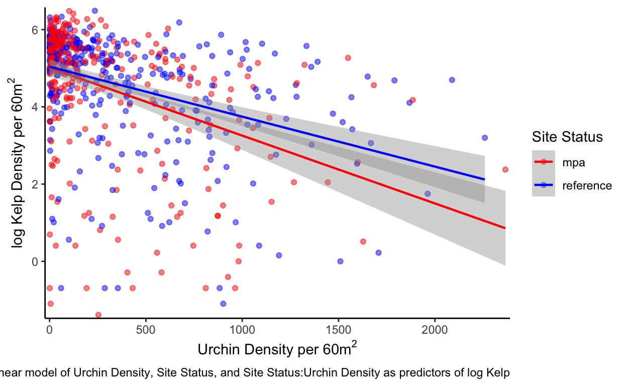
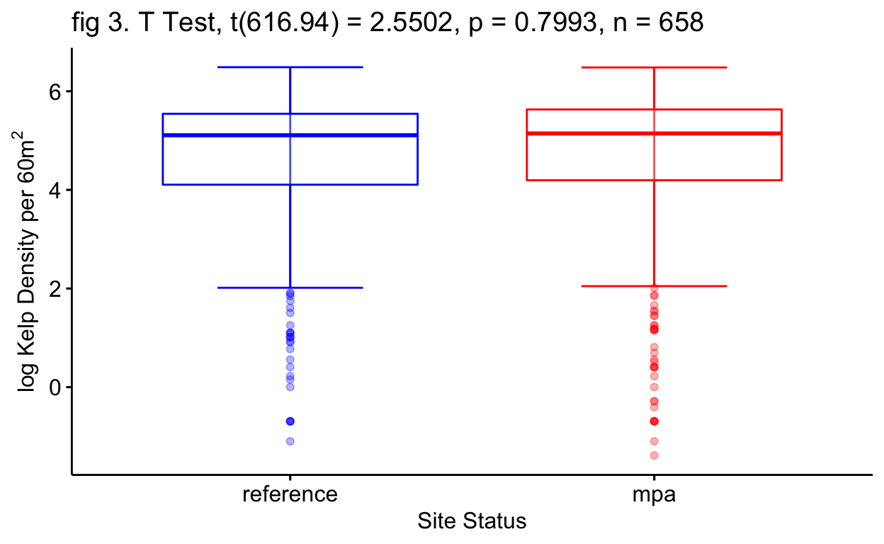
To determine what might be the cause of these differences of kelp densities in the MPAs and reference sites, a linear model was created (\(\alpha\) < 0.05) (Tbl 1, fig 3). Annual site means for urchin densities, site status (MPA or Reference Site), and site status as an interaction with urchin densities, were all used as predictors for log kelp densities in the linear model. The results illustrate that urchin density is a significant predictor for log kelp densities (p<0.001). Interestingly site status is a poor predictor for log kelp densities (p=0.845) yet anecdotal observations say otherwise. The urchin density and site status interaction (p=0.095) was not found to be a significant interaction but can still indicate the affects that can occur between the two predictors. A negative trend can clearly be seen between log kelp density and urchin densities (fig 3). Overall model predictability is rather low (adjusted \(R^{2}\) = 0.154) and not suited for predicting log kelp variability.
hide
mod <- lm(log_mac ~ den_STRPURAD + site_status + site_status:den_STRPURAD,
        data = annual_mean)

tab_model(mod,
          pred.labels = c("Intercept", "Urchin Density", "Site Status",
                          "Urchin Density:Site Status"),
          dv.labels = c("log Kelp Density"),
          string.ci = "Conf. Int (95%)",
          string.p = "P-value",
          title = "Tbl 1. Linear Model Results for Below Predictors",
          digits = 4)
| log Kelp Density | |||
|---|---|---|---|
| Predictors | Estimates | Conf. Int (95%) | P-value |
| Intercept | 5.0113 | 4.8108 – 5.2119 | <0.001 |
| Urchin Density | -0.0018 | -0.0022 – -0.0013 | <0.001 |
| Site Status | 0.0280 | -0.2529 – 0.3088 | 0.845 |
| Urchin Density:Site Status | 0.0005 | -0.0001 – 0.0010 | 0.095 |
| Observations | 658 | ||
| R2 / R2 adjusted | 0.158 / 0.154 | ||
hide
annual_mean %>%
  ggplot(aes(x = den_STRPURAD, y = log_mac, color = site_status)) +
  geom_point(alpha = 0.5, aes(color =site_status)) +
  geom_smooth(formula = y ~ x, method = "lm", se = T, lwd = 0.8) +
  theme_classic() +
  scale_y_continuous(expand = c(0.01,0.01)) +
  scale_x_continuous(expand = c(0.01,0.01)) +
  ylab(expression("log Kelp Density per 60m"^2)) +
  xlab(expression("Urchin Density per 60m"^2)) +
  labs(color = "Site Status",
       caption = "fig 3. Linear model of Urchin Density, Site Status, and Site Status:Urchin Density as predictors of log Kelp") +
  scale_color_manual(values = c("red", "blue"))
Welch Two Sample T Test
In order to test my anecdotal evidence of higher densities of kelp and lower densities of urchins in the MPAs and vice versa for reference sites, I have created a set of Welch Two Sample t-tests (\(\alpha\) < 0.05).
The null hypothesis: There is no difference of kelp and urchin densities between MPAs and reference sites for the selected data set.
The alternative hypothesis: There is a difference in kelp and urchin densities between MPAs and reference sites for the selected data set.
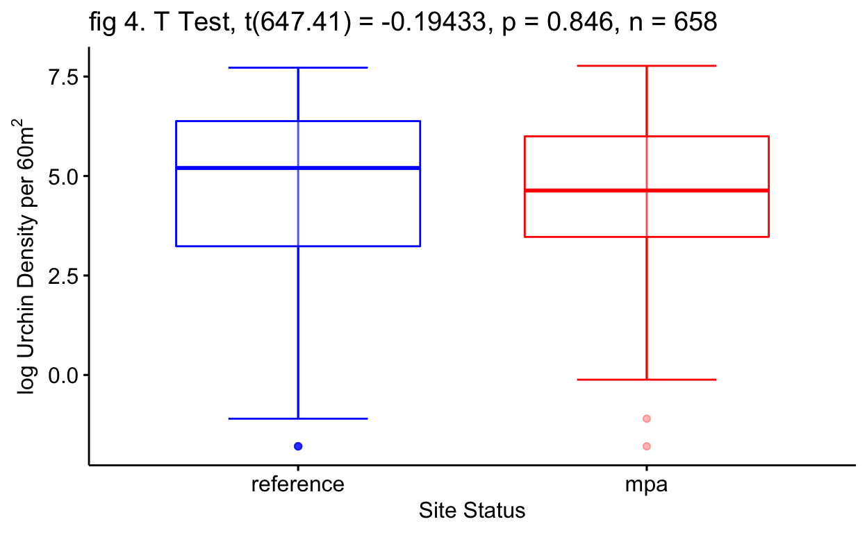
The first t-test concluded that we would fail to reject the null hypothesis of site status as a predictor for log kelp density (p=0.675) (fig 3 Tbl 2). The second t-test once again concluded that we would fail to reject the null hypothesis of site status as a predictor for log urchin density (p=0.846) (fig 4 Tbl 3). This may not align with my current anecdotal evidence and that is understandable as these t-tests include many data points through time that counter my current anecdotal evidence (fig 2).
hide
#null: no difference of kelp and urchins across reference sites and mpas

#alternative: there is a difference


kelp.test <-t.test(log_mac ~ site_status, data = annual_mean)


tab_model(kelp.test,
          string.ci = c("Conf. Int (95%)"),
          string.p = "P-value",
          dv.labels = c("log Kelp Density"),
          pred.labels = "Site Status",
          title = "Tbl 2. log Kelp Welch Two Sample t-test")
| log Kelp Density | |||
|---|---|---|---|
| Predictors | Estimates | Conf. Int (95%) | P-value |
| Site Status | -0.05 | -0.30 – 0.19 | 0.675 |
hide
kelp_boxp <- ggboxplot(annual_mean, x = "site_status", y = "log_mac",
                     xlab = "Site Status", ylab = expression("log Kelp Density per 60m"^2),
                     title = "fig 3. T Test, t(616.94) = 2.5502, p = 0.7993, n = 658",
                     bxp.errorbar = T,
                     alpha = 0.3,
                     color = c("blue", "red"))


kelp_boxp
hide
| log Urchin Density | |||
|---|---|---|---|
| Predictors | Estimates | Conf. Int (95%) | P-value |
| Site Status | -0.03 | -0.34 – 0.28 | 0.846 |
hide
urch_bxp <-ggboxplot(annual_mean, x = "site_status", y = "log_urch",
                     xlab = "Site Status", ylab = expression("log Urchin Density per 60m"^2),
                     title = "fig 4. T Test, t(647.41) = -0.19433, p = 0.846, n = 658",
                     bxp.errorbar = T,
                     alpha = 0.3,
                     color = c("blue", "red"))


urch_bxp
MPA Implementation Linear Model
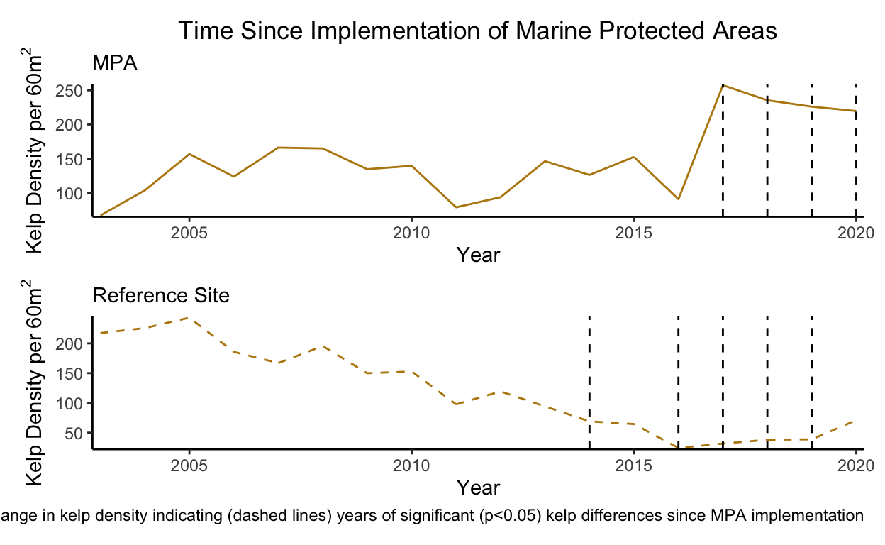
In order to test the affects of time since MPA implementation on kelp densities both in MPAs and reference sites a linear model was created with time since MPA implementation as a predictor for log kelp densities (Tbl 4 & 5). A significant difference (\(\alpha\) < 0.05) in kelp densities since the implementation of the MPAs occurred for years 15-18 (p=0.019, 0.012, 0.008, 0.01) after implementation or 2017-2020 (fig 6 Tbl 4).
A similar trend occurred for the reference sites. A significant difference in kelp densities since the implementation of MPAs occurred 12, 14-17 (p=0.001, <0.001, <0.001, 0.002, <0.001) years after implementation or 2014, 2016, 2017-2019.
hide
time_lag_mpa <- annual_mean %>%
  filter(site_status == "mpa",
         survey_year >2000)%>%
  group_by(survey_year) %>%
  add_column(time_mpa = "")

time_lag_mpa$time_mpa <- cut(time_lag_mpa$survey_year,
                             c(2002:2020), c(1:18))

time_lag_mpa <- time_lag_mpa %>%
   filter(survey_year > 2002)


mpa_mod <- lm(log_mac ~ time_mpa,
              data = time_lag_mpa)

tab_model(mpa_mod, df.method = "kr",
          string.ci = "Conf. Int (95%)",
          string.p = "P-value",
          pred.labels = c("Intercept", "2 Years", "3 Years", "4 Years", "5 Years", "6 Years",
                          "7 Years", "8 Years", "9 Years", "10 Years", "11 Years", "12 Years", "13 Years", "14 Years",
                          "15 Years", "16 Years", "17 Years", "18 Years"),
          dv.labels = c("log Kelp Density"),
          title = "Tbl 4 Linear model fit for change in MPA kelp density since implementation")
| log Kelp Density | |||
|---|---|---|---|
| Predictors | Estimates | Conf. Int (95%) | P-value |
| Intercept | 3.86 | 2.90 – 4.81 | <0.001 |
| 2 Years | 0.22 | -1.13 – 1.56 | 0.751 |
| 3 Years | 0.39 | -0.83 – 1.60 | 0.532 |
| 4 Years | 0.77 | -0.57 – 2.12 | 0.259 |
| 5 Years | 0.78 | -0.40 – 1.96 | 0.195 |
| 6 Years | 0.23 | -0.96 – 1.42 | 0.707 |
| 7 Years | 0.23 | -0.92 – 1.39 | 0.690 |
| 8 Years | 0.88 | -0.37 – 2.12 | 0.166 |
| 9 Years | -0.06 | -1.33 – 1.22 | 0.931 |
| 10 Years | 0.36 | -0.93 – 1.66 | 0.583 |
| 11 Years | 0.45 | -0.92 – 1.83 | 0.518 |
| 12 Years | 0.25 | -0.98 – 1.48 | 0.691 |
| 13 Years | 0.88 | -0.37 – 2.14 | 0.168 |
| 14 Years | -0.26 | -1.52 – 0.99 | 0.680 |
| 15 Years | 1.49 | 0.25 – 2.73 | 0.019 |
| 16 Years | 1.60 | 0.36 – 2.84 | 0.012 |
| 17 Years | 1.71 | 0.45 – 2.96 | 0.008 |
| 18 Years | 1.67 | 0.41 – 2.92 | 0.010 |
| Observations | 296 | ||
| R2 / R2 adjusted | 0.120 / 0.066 | ||
hide
time_lag_ref <- annual_mean %>%
  filter(site_status == "reference",
         survey_year >2000)%>%
  group_by(survey_year) %>%
  add_column(time_ref = "")

time_lag_ref$time_ref <- cut(time_lag_ref$survey_year,
                             c(2002:2020), c(1:18))

time_lag_ref <- time_lag_ref %>%
   filter(survey_year > 2002)

ref_mod <- lm(log_mac ~ time_ref,
              data = time_lag_ref)

tab_model(ref_mod, df.method = "kr",
          string.ci = "Conf. Int (95%)",
          string.p = "P-value",
          pred.labels = c("Intercept", "2 Years", "3 Years", "4 Years", "5 Years", "6 Years",
                          "7 Years", "8 Years", "9 Years", "10 Years", "12 Years", "13 Years", "14 Years",
                          "15 Years", "16 Years", "17 Years", "18 Years"),
          dv.labels = c("log Kelp Density"),
          title = "Tbl 5. Linear model fit for change in reference site kelp density since implementation")
| log Kelp Density | |||
|---|---|---|---|
| Predictors | Estimates | Conf. Int (95%) | P-value |
| Intercept | 5.03 | 4.36 – 5.70 | <0.001 |
| 2 Years | 0.54 | -0.34 – 1.43 | 0.228 |
| 3 Years | 0.39 | -0.48 – 1.26 | 0.377 |
| 4 Years | 0.07 | -0.82 – 0.95 | 0.880 |
| 5 Years | 0.23 | -0.58 – 1.03 | 0.577 |
| 6 Years | 0.04 | -0.77 – 0.85 | 0.929 |
| 7 Years | 0.05 | -0.75 – 0.85 | 0.907 |
| 8 Years | -0.21 | -1.03 – 0.61 | 0.614 |
| 9 Years | -0.65 | -1.48 – 0.19 | 0.127 |
| 10 Years | -0.34 | -1.18 – 0.50 | 0.429 |
| 12 Years | -1.50 | -2.39 – -0.62 | 0.001 |
| 13 Years | -0.99 | -1.99 – 0.00 | 0.051 |
| 14 Years | -2.23 | -3.20 – -1.26 | <0.001 |
| 15 Years | -2.10 | -3.05 – -1.14 | <0.001 |
| 16 Years | -1.47 | -2.39 – -0.55 | 0.002 |
| 17 Years | -1.71 | -2.63 – -0.78 | <0.001 |
| 18 Years | -0.83 | -1.80 – 0.14 | 0.094 |
| Observations | 332 | ||
| R2 / R2 adjusted | 0.303 / 0.267 | ||
hide
kelp_time_mpa <- ggplot(data = time_lag_mpa) +
  geom_line(aes(x = survey_year, y = mean_stipe), color = "darkgoldenrod") +
  theme_classic()+
  xlab("Year")+
  ylab(expression("Kelp Density per 60m"^2)) +
  labs(color = "Site Status") +
  geom_vline(xintercept = 2018, linetype = "dashed")+
  geom_vline(xintercept = 2019, linetype = "dashed")+
  geom_vline(xintercept = 2017, linetype = "dashed") +
  geom_vline(xintercept = 2020, linetype = "dashed") +
  scale_alpha_continuous()+
  scale_y_continuous(expand = c(0.01,0.01)) +
  scale_x_continuous(expand = c(0.01,0.01)) +
  labs(title = "Time Since Implementation of Marine Protected Areas", subtitle = "MPA") +
  theme(plot.title = element_text(hjust = 0.5))


kelp_time_ref <- ggplot(data = time_lag_ref) +
  geom_line(aes(x = survey_year, y = mean_stipe),
            color = "darkgoldenrod", linetype = "dashed") +
  theme_classic()+
  xlab("Year")+
  ylab(expression("Kelp Density per 60m"^2)) +
  labs(color = "Site Status") +
  geom_vline(xintercept = 2017, linetype = "dashed")+
  geom_vline(xintercept = 2018, linetype = "dashed")+
  geom_vline(xintercept = 2019, linetype = "dashed") +
  geom_vline(xintercept = 2016, linetype = "dashed") +
  geom_vline(xintercept = 2014, linetype = "dashed") +
  scale_y_continuous(expand = c(0.01,0.01)) +
  scale_x_continuous(expand = c(0.01,0.01)) +
  labs(subtitle = "Reference Site",
       caption = "fig 6. Change in kelp density indicating (dashed lines) years of significant (p<0.05) kelp differences since MPA implementation")

kelp_time_mpa / kelp_time_ref
Discussion
Understanding the changes that occur from the implementation of MPAs is important so we can know if they are working and benefiting the ecosystem. Through long term monitoring and analysis we can better understand how they evolve through time and this knowledge can then be translated across regions and systems for the implementation of new MPAs or reserves.
From these results we can see changes in kelp densities from the implementation of MPAs are not explicitly evident (fig 2). Kelp forests are highly dynamic ecosystems and fluctuations caused through environmental changes can lead to challenges in understanding changes through time (fig 2) (Reed et al. 2014). However from our linear models there does seem to be strong evidence of a negative relationship between urchin densities and kelp densities (fig 3 Tbl 1). This significant result (\(\alpha\) < 0.05) does line up with my own anecdotal evidence of survey sites with high urchin densities and low kelp density or vice versa. Interestingly, I did not see any evidence for site status to significantlly affect either kelp or urchin densities (fig 3, 4, 5 Tbl 1,2,3). However, based on the long-run trends of urchin and kelp densities this makes sense why the tests I conducted did not pick up a difference (fig 2). There was a long period of time, many data points, where kelp densities did not significantly differ between MPAs and reference sites (fig 6 Tbl 4,5). The time period at which kelp densities began to significantly differ between MPAs and reference sites coincides with my own anecdotal observations beginning in 2017 (fig 6, Tbl 4,5) as that is when I began conducting surveys for PISCO.
With the supporting figures showing mixed results of support for model choice, it is important to point out that random sampling was conducted, residual mean is near zero, and error terms are normally distributed. However there is heteroscedasticity and the qqplot is not linear.
Now the real question lies with in, what happened in the year 2013-2014 at the N. Channel Islands that caused such sudden changes in kelp and urchin densities inside MPAs and reference sites (fig 2)? Further research needs to be conducted but evidence supports that the mass sea star war wasting event that proliferated from Baja to Alaska affected kelp densities (Eisaguirre et al., 2020). The sunflower star (Pycnopodia helianthordes), a keystone species, consumes urchins but was functionally extirpated from the N. Channel Islands by 2014 due to sea star wasting disease (Eisaguirre et al., 2020, Hewson et al., 2018, Moitoza & Philips, 1979) . A change as abrupt and sudden as the loss of a keystone species can cause shifts in any ecosystem. Especially if a site (IE reference site) is heavily fished, thus decreasing the remaining urchin predator guild, and ultimately leading to an explosion of urchins with a dramatic loss of kelp (Eisaguirre et al., 2020). However if a site is protected, the release of fishing pressure can lead to increased resilience in the system due to the remaining urchin predator guild mediating urchin levels and allowing for kelp’s to persist (Eisaguirre et al., 2020).
Conclusion
Further research needs to be conducted, however this study lends support to the importance of maintaining urchin populations in order for healthy kelp forests to persist. Along with the idea that kelps in marine protected areas could possibly withstand a greater degree of perturbations supporting the already hypothesized theory that MPAs increase ecosystem resilience.
References
Channel Keeper. “About the Santa Barbara Channel.” About the Santa Barbara Channel, November 27, 2021. https://www.sbck.org/about-us/about-the-santa-barbara-channel/.
Eisaguirre, Jacob H., Joseph M.Eisaguirre, Kathryn Davis, Peter M. Carlson, Steven D. Gaines, and Jennifer E. Caselle. “Trophic Redundancy and Predator Size Class Structure Drive Differences in Kelp Forest Ecosystem Dynamics.” Ecology 101, no. 5 (2020): e02993. https://doi.org/10.1002/ecy.2993.
Filbee-Dexter, K, and Re Scheibling. “Sea Urchin Barrens as Alternative Stable States of Collapsed Kelp Ecosystems.” Marine Ecology Progress Series 495 (January 9, 2014): 1–25. https://doi.org/10.3354/meps10573.
Hamilton, Scott L., and Jennifer E. Caselle. “Exploitation and Recovery of a Sea Urchin Predator Has Implications for the Resilience of Southern California Kelp Forests.” Proceedings of the Royal Society B: Biological Sciences 282, no. 1799 (January 22, 2015): 20141817. https://doi.org/10.1098/rspb.2014.1817.
Hewson, Ian, Kalia S. I. Bistolas, Eva M. Quijano Cardé, Jason B. Button, Parker J. Foster, Jacob M. Flanzenbaum, Jan Kocian, and Chaunte K. Lewis. “Investigating the Complex Association Between Viral Ecology, Environment, and Northeast Pacific Sea Star Wasting.” Frontiers in Marine Science 5 (2018): 77. https://doi.org/10.3389/fmars.2018.00077.
Ling, S. D., R. E. Scheibling, A. Rassweiler, C. R. Johnson, N. Shears, S. D. Connell, A. K. Salomon, et al. “Global Regime Shift Dynamics of Catastrophic Sea Urchin Overgrazing.” Philosophical Transactions of the Royal Society B: Biological Sciences 370, no. 1659 (January 5, 2015): 20130269. https://doi.org/10.1098/rstb.2013.0269.
Moitoza, D. J., and D. W. Phillips. “Prey Defense, Predator Preference, and Nonrandom Diet: The Interactions between Pycnopodia Helianthoides and Two Species of Sea Urchins.” Marine Biology 53, no. 4 (August 1, 1979): 299–304. https://doi.org/10.1007/BF00391611.
“Prey Defense, Predator Preference, and Nonrandom Diet: The Interactions between Pycnopodia Helianthoides and Two Species of Sea Urchins.” Marine Biology 53, no. 4 (August 1, 1979): 299–304. https://doi.org/10.1007/BF00391611.
Reed, Daniel C., Andrew R. Rassweiler, Robert J. Miller, Henry M. Page, Sally J. Holbrook, Daniel C. Reed, Andrew R. Rassweiler, Robert J. Miller, Henry M. Page, and Sally J. Holbrook. “The Value of a Broad Temporal and Spatial Perspective in Understanding Dynamics of Kelp Forest Ecosystems.” Marine and Freshwater Research 67, no. 1 (July 6, 2015): 14–24. https://doi.org/10.1071/MF14158.
Selden, Rebecca L., Steven D. Gaines, Scott L. Hamilton, and Robert R. Warner. “Protection of Large Predators in a Marine Reserve Alters Size-Dependent Prey Mortality.” Proceedings of the Royal Society B: Biological Sciences 284, no. 1847 (January 25, 2017): 20161936. https://doi.org/10.1098/rspb.2016.1936.
“Marine Protected Areas - Channel Islands National Park (U.S. National Park Service).” National Park Service. Accessed November 27, 2021. https://www.nps.gov/chis/learn/nature/marine-protected-areas.htm.
Supporting Figures
GitHub Repository: https://github.com/Jake-Eisaguirre/Final_Project
hide
urch_dist <- ggplot(data = annual_mean) +
  geom_histogram(aes(den_STRPURAD), binwidth = 70) +
  theme_classic() +
  xlab(expression("Urchin Density per 60m"^2)) +
  labs(caption = "Distribution of dependent variables")


mac_dist <- ggplot(data = annual_mean) +
  geom_histogram(aes(den_MACSTIPES), binwidth = 15) +
  theme_classic() +
  xlab(expression("Kelp Density per 60m"^2))

urch_dist * mac_dist
hide
caption =
# Log Transformed Normality
log_urch_dist <- ggplot(data = annual_mean) +
  geom_histogram(aes(log_urch), binwidth = 0.15) +
  theme_classic() +
  xlab("log Urchins") +
    labs(caption = "Log transformed distribution of dependent variables")


log_mac_dist <- ggplot(data = annual_mean) +
  geom_histogram(aes(log_mac), binwidth = 0.15) +
  theme_classic() +
  xlab("log Kelp")

log_urch_dist * log_mac_dist
hide
# Model Fit

aug <- annual_mean %>%
  add_predictions(mod) %>%
  mutate(residuals_mac = log_mac - pred)


ggplot(data = aug) +
  geom_histogram(aes(residuals_mac), binwidth = 0.25) +
  theme_classic() +
  xlab("Kelp Residuals")
hide
qqPlot(aug$residuals_mac)
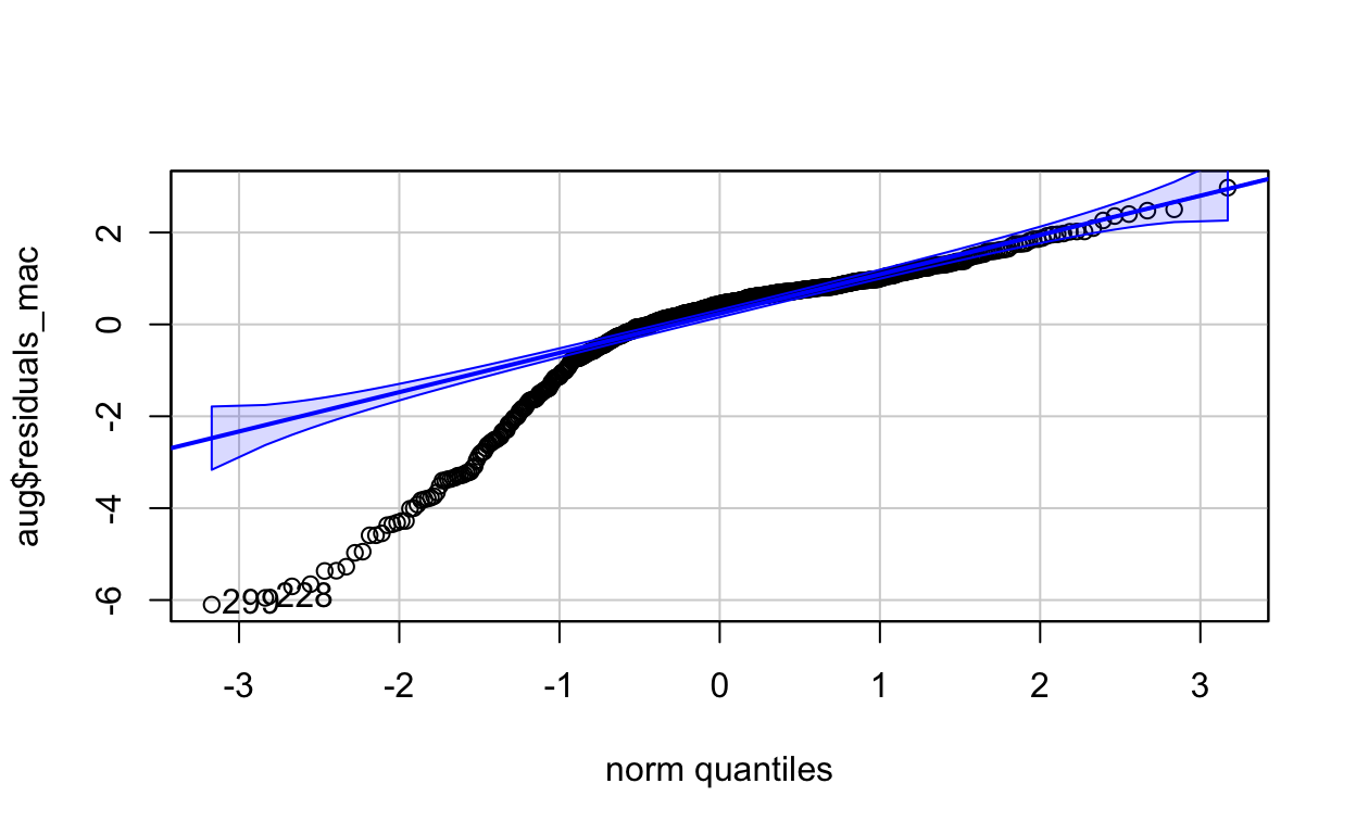
[1] 299 228hide
ggplot(data = aug) +
  geom_point(aes(y = residuals_mac, x = den_STRPURAD), alpha = 0.3) +
  geom_hline(yintercept = 0, linetype = "dashed") +
  theme_classic() +
  xlab(expression("Urchin Density per 60m"^2)) +
  ylab("Kelp Residuals")