# load packages, installing if missing
if (!require(librarian)){
install.packages("librarian")
library(librarian)
}
.libPaths(c(.libPaths(), "/Users/bbest/R/x86_64-pc-linux-gnu-library/4.0"))
librarian::shelf(
raster, dismo, dplyr, DT, ggplot2, here, htmltools, leaflet, mapview, purrr, readr, rgbif, rgdal, rJava, sdmpredictors, sf, spocc, tidyr, geojsonio)
select <- dplyr::select # overwrite raster::select
# set random seed for reproducibility
set.seed(42)
# directory to store data
dir_data <- here("data/sdm")
dir.create(dir_data, showWarnings = F)
obs_csv <- here("obs.csv")
obs_geo <- here("obs.geojson")
# get species occurrence data from GBIF with coordinates
(res <- spocc::occ(
query = 'Cervus canadensis',
from = 'gbif', has_coords = T,
limit = 12000))
Searched: gbif
Occurrences - Found: 12,156, Returned: 12,000
Search type: Scientific
gbif: Cervus canadensis (12000)# extract data frame from result
df <- res$gbif$data[[1]]
nrow(df) # number of rows
[1] 12000# convert to points of observation from lon/lat columns in data frame
obs <- df %>%
filter(longitude < 0) %>% #<- North America Only
select("longitude", "latitude") %>%
sf::st_as_sf(
coords = c("longitude", "latitude"),
crs = st_crs(4326))
readr::write_csv(df, obs_csv)
geojsonio::geojson_write(obs, obs_geo)
<geojson-file>
Path: myfile.geojson
From class: geo_list# show points on map
mapview::mapview(obs, map.types = "Esri.WorldImagery")
dir_env <- here("env")
# set a default data directory
options(sdmpredictors_datadir = dir_env)
# choosing terrestrial
env_datasets <- sdmpredictors::list_datasets(terrestrial = TRUE, marine = FALSE)
# show table of datasets
env_datasets %>%
select(dataset_code, description, citation) %>%
DT::datatable()
# choose datasets for a vector
env_datasets_vec <- c("WorldClim", "ENVIREM")
# get layers
env_layers <- sdmpredictors::list_layers(env_datasets_vec)
DT::datatable(env_layers)
# choose layers after some inspection and perhaps consulting literature
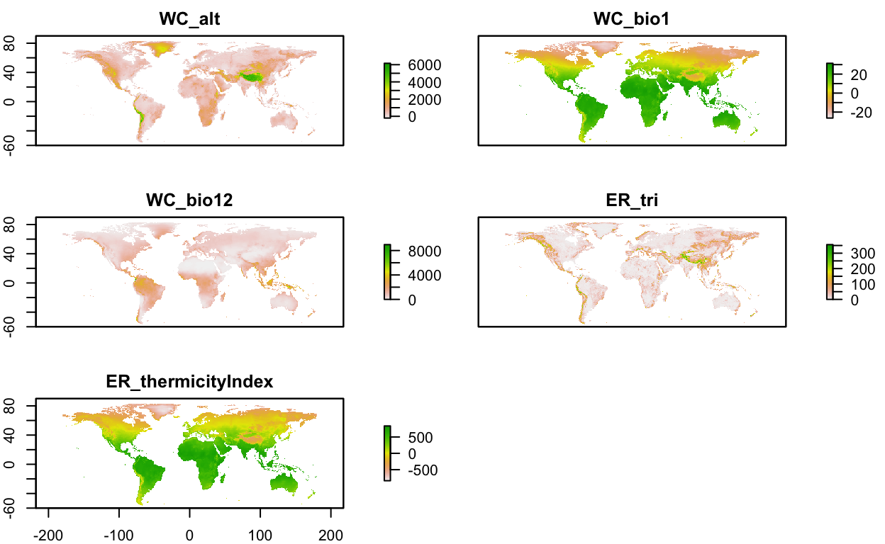
env_layers_vec <- c("WC_alt", "WC_bio1", "WC_bio12", "ER_tri", "ER_thermicityIndex")
# get layers
env_stack <- load_layers(env_layers_vec)
# interactive plot layers, hiding all but first (select others)
#mapview(env_stack, hide = T)
plot(env_stack, nc=2)
obs_hull_geo <- here("obs_hull.geojson")
# make convex hull around points of observation
obs_hull <- sf::st_convex_hull(st_union(obs))
# show points on map
mapview(
list(obs, obs_hull))
# save obs hull
write_sf(obs_hull, obs_hull_geo)
obs_hull_sp <- sf::as_Spatial(obs_hull)
env_stack <- raster::mask(env_stack, obs_hull_sp) %>%
raster::crop(extent(obs_hull_sp))
mapview(obs) +
mapview(env_stack, hide = T)
absence_geo <- here("absence.geojson")
pts_geo <- here("pts.geojson")
pts_env_csv <- here("pts_env.csv")
# get raster count of observations
r_obs <- rasterize(
sf::as_Spatial(obs), env_stack[[1]], field=1, fun='count')
mapview(obs) +
mapview(r_obs)
# create mask for
r_mask <- mask(env_stack[[1]] > -Inf, r_obs, inverse=T)
absence <- dismo::randomPoints(r_mask, nrow(obs)) %>%
as_tibble() %>%
st_as_sf(coords = c("x", "y"), crs = 4326)
mapview(obs, col.regions = "green") +
mapview(absence, col.regions = "gray")
# combine presence and absence into single set of labeled points
pts <- rbind(
obs %>%
mutate(
present = 1) %>%
select(present),
absence %>%
mutate(
present = 0)) %>%
mutate(
ID = 1:n()) %>%
relocate(ID)
write_sf(pts, pts_geo)
# extract raster values for points
pts_env <- raster::extract(env_stack, as_Spatial(pts), df=TRUE) %>%
tibble() %>%
# join present and geometry columns to raster value results for points
left_join(
pts %>%
select(ID, present),
by = "ID") %>%
relocate(present, .after = ID) %>%
# extract lon, lat as single columns
mutate(
#present = factor(present),
lon = st_coordinates(geometry)[,1],
lat = st_coordinates(geometry)[,2]) %>%
select(-geometry)
write_csv(pts_env, pts_env_csv)
pts_env %>%
select(-ID) %>%
mutate(
present = factor(present)) %>%
pivot_longer(-present) %>%
ggplot() +
geom_density(aes(x = value, fill = present)) +
scale_fill_manual(values = alpha(c("gray", "green"), 0.5)) +
scale_x_continuous(expand=c(0,0)) +
scale_y_continuous(expand=c(0,0)) +
theme_bw() +
facet_wrap(~name, scales = "free") +
theme(
legend.position = c(1, 0),
legend.justification = c(1, 0))

pts_env_csv <- here("pts_env.csv")
pts_env <- read_csv(pts_env_csv)
nrow(pts_env)
[1] 23778datatable(pts_env, rownames = F)

# setup model data
d <- pts_env %>%
# # remove terms we don't want to model
tidyr::drop_na() # drop the rows with NA values
nrow(d)
[1] 23735
Call:
lm(formula = present ~ ., data = d)
Residuals:
Min 1Q Median 3Q Max
-0.80576 -0.16523 0.00631 0.17184 0.67036
Coefficients:
Estimate Std. Error t value Pr(>|t|)
(Intercept) 2.193e+00 4.321e-02 50.76 <2e-16 ***
ID -5.442e-05 2.501e-07 -217.56 <2e-16 ***
WC_alt -1.139e-04 6.731e-06 -16.92 <2e-16 ***
WC_bio1 -2.618e-02 1.399e-03 -18.72 <2e-16 ***
WC_bio12 6.933e-05 3.906e-06 17.75 <2e-16 ***
ER_tri 5.197e-04 4.431e-05 11.73 <2e-16 ***
ER_thermicityIndex -6.697e-04 5.635e-05 -11.88 <2e-16 ***
lon -7.547e-03 2.104e-04 -35.87 <2e-16 ***
lat -3.727e-02 1.034e-03 -36.04 <2e-16 ***
---
Signif. codes: 0 '***' 0.001 '**' 0.01 '*' 0.05 '.' 0.1 ' ' 1
Residual standard error: 0.2277 on 23726 degrees of freedom
Multiple R-squared: 0.7927, Adjusted R-squared: 0.7926
F-statistic: 1.134e+04 on 8 and 23726 DF, p-value: < 2.2e-16# show term plots
termplot(mdl, partial.resid = TRUE, se = TRUE, main = F)


# fit a generalized linear model with a binomial logit link function
mdl <- glm(present ~ ., family = binomial(link="logit"), data = d)
summary(mdl)
Call:
glm(formula = present ~ ., family = binomial(link = "logit"),
data = d)
Deviance Residuals:
Min 1Q Median 3Q Max
-0.03401 0.00000 0.00000 0.00000 0.01937
Coefficients:
Estimate Std. Error z value Pr(>|z|)
(Intercept) 1.129e+04 2.102e+04 0.537 0.591
ID -9.628e-01 1.786e+00 -0.539 0.590
WC_alt 1.692e-02 1.581e-01 0.107 0.915
WC_bio1 4.455e+00 4.331e+01 0.103 0.918
WC_bio12 3.212e-02 1.225e-01 0.262 0.793
ER_tri -1.070e-01 1.090e+00 -0.098 0.922
ER_thermicityIndex -1.449e-01 1.610e+00 -0.090 0.928
lon -1.012e+00 5.835e+00 -0.173 0.862
lat -3.547e-01 2.250e+01 -0.016 0.987
(Dispersion parameter for binomial family taken to be 1)
Null deviance: 3.2904e+04 on 23734 degrees of freedom
Residual deviance: 2.8995e-03 on 23726 degrees of freedom
AIC: 18.003
Number of Fisher Scoring iterations: 25librarian::shelf(mgcv)
# fit a generalized additive model with smooth predictors
mdl <- mgcv::gam(
formula = present ~ s(WC_alt) + s(WC_bio1) +
s(WC_bio12) + s(ER_tri) + s(ER_thermicityIndex) + s(lon) + s(lat),
family = binomial, data = d)
summary(mdl)
Family: binomial
Link function: logit
Formula:
present ~ s(WC_alt) + s(WC_bio1) + s(WC_bio12) + s(ER_tri) +
s(ER_thermicityIndex) + s(lon) + s(lat)
Parametric coefficients:
Estimate Std. Error z value Pr(>|z|)
(Intercept) -0.30271 0.04773 -6.342 2.27e-10 ***
---
Signif. codes: 0 '***' 0.001 '**' 0.01 '*' 0.05 '.' 0.1 ' ' 1
Approximate significance of smooth terms:
edf Ref.df Chi.sq p-value
s(WC_alt) 8.617 8.951 934.9 <2e-16 ***
s(WC_bio1) 8.990 8.999 259.8 <2e-16 ***
s(WC_bio12) 8.902 8.992 419.2 <2e-16 ***
s(ER_tri) 8.212 8.807 1283.5 <2e-16 ***
s(ER_thermicityIndex) 8.140 8.746 554.8 <2e-16 ***
s(lon) 8.910 8.997 771.6 <2e-16 ***
s(lat) 8.942 8.999 742.2 <2e-16 ***
---
Signif. codes: 0 '***' 0.001 '**' 0.01 '*' 0.05 '.' 0.1 ' ' 1
R-sq.(adj) = 0.61 Deviance explained = 52.6%
UBRE = -0.3374 Scale est. = 1 n = 23735# show term plots
plot(mdl, scale=0)


# load extra packages
librarian::shelf(
maptools, sf)
# show version of maxent
maxent()
This is MaxEnt version 3.4.3 
# get presence-only observation points (maxent extracts raster values for you)
obs_sp <- read_sf(here("_posts", "2022-01-19-mlelk", "obs.geojson")) %>%
sf::as_Spatial() # maxent prefers sp::SpatialPoints over newer sf::sf class
# fit a maximum entropy model
mdl <- maxent(env_stack, obs_sp)
This is MaxEnt version 3.4.3 # plot variable contributions per predictor
plot(mdl)

# plot term plots
response(mdl)

# predict
y_predict <- predict(env_stack, mdl) #, ext=ext, progress='')
plot(y_predict, main='Maxent, raw prediction')
data(wrld_simpl, package="maptools")
plot(wrld_simpl, add=TRUE, border='dark grey')

# global knitr chunk options
knitr::opts_chunk$set(
warning = FALSE,
message = FALSE)
# load packages
librarian::shelf(
caret, # m: modeling framework
dplyr, ggplot2 ,here, readr,
pdp, # X: partial dependence plots
rpart, # m: recursive partition modeling
rpart.plot, # m: recursive partition plotting
rsample, # d: split train/test data
skimr, # d: skim summarize data table
vip) # X: variable importance
# options
options(
scipen = 999,
readr.show_col_types = F)
set.seed(42)
# graphical theme
ggplot2::theme_set(ggplot2::theme_light())
# paths
dir_data <- here("data/sdm")
pts_env_csv <- here("pts_env.csv")
# read data
pts_env <- read_csv(pts_env_csv)
d <- pts_env %>%
select(-ID) %>% # not used as a predictor x
mutate(
present = factor(present)) %>% # categorical response
na.omit() # drop rows with NA
skim(d)
| Name | d |
| Number of rows | 23735 |
| Number of columns | 8 |
| _______________________ | |
| Column type frequency: | |
| factor | 1 |
| numeric | 7 |
| ________________________ | |
| Group variables | None |
Variable type: factor
| skim_variable | n_missing | complete_rate | ordered | n_unique | top_counts |
|---|---|---|---|---|---|
| present | 0 | 1 | FALSE | 2 | 0: 11879, 1: 11856 |
Variable type: numeric
| skim_variable | n_missing | complete_rate | mean | sd | p0 | p25 | p50 | p75 | p100 | hist |
|---|---|---|---|---|---|---|---|---|---|---|
| WC_alt | 0 | 1 | 1185.84 | 928.34 | -73.00 | 332.00 | 986.00 | 2010.50 | 3652.00 | ▇▅▃▃▁ |
| WC_bio1 | 0 | 1 | 7.02 | 5.88 | -11.70 | 2.10 | 7.20 | 11.00 | 23.30 | ▁▅▇▆▂ |
| WC_bio12 | 0 | 1 | 754.26 | 500.13 | 53.00 | 436.00 | 584.00 | 925.00 | 4508.00 | ▇▂▁▁▁ |
| ER_tri | 0 | 1 | 50.68 | 48.22 | 0.00 | 9.71 | 36.24 | 79.96 | 321.60 | ▇▃▁▁▁ |
| ER_thermicityIndex | 0 | 1 | 56.95 | 171.32 | -496.75 | -77.25 | 56.00 | 189.75 | 519.50 | ▁▅▇▆▁ |
| lon | 0 | 1 | -108.43 | 12.91 | -144.38 | -118.07 | -110.38 | -101.79 | -74.46 | ▁▅▇▃▂ |
| lat | 0 | 1 | 42.57 | 7.29 | 27.12 | 36.62 | 41.38 | 46.96 | 63.62 | ▂▇▆▃▁ |
# create training set with 80% of full data
d_split <- rsample::initial_split(d, prop = 0.8, strata = "present")
d_train <- rsample::training(d_split)
# show number of rows present is 0 vs 1
table(d$present)
0 1
11879 11856 # run decision stump model
mdl <- rpart(
present ~ ., data = d_train,
control = list(
cp = 0, minbucket = 5, maxdepth = 1))
mdl
n= 18987
node), split, n, loss, yval, (yprob)
* denotes terminal node
1) root 18987 9484 0 (0.5005003 0.4994997)
2) ER_tri< 19.345 7005 995 0 (0.8579586 0.1420414) *
3) ER_tri>=19.345 11982 3493 1 (0.2915206 0.7084794) *
# decision tree with defaults
mdl <- rpart(present ~ ., data = d_train)
mdl
n= 18987
node), split, n, loss, yval, (yprob)
* denotes terminal node
1) root 18987 9484 0 (0.50050034 0.49949966)
2) ER_tri< 19.345 7005 995 0 (0.85795860 0.14204140)
4) WC_alt< 1972 6672 735 0 (0.88983813 0.11016187)
8) lon>=-120.571 6183 416 0 (0.93271874 0.06728126) *
9) lon< -120.571 489 170 1 (0.34764826 0.65235174)
18) WC_bio1< 8.7 153 18 0 (0.88235294 0.11764706) *
19) WC_bio1>=8.7 336 35 1 (0.10416667 0.89583333) *
5) WC_alt>=1972 333 73 1 (0.21921922 0.78078078) *
3) ER_tri>=19.345 11982 3493 1 (0.29152061 0.70847939)
6) lat>=53.19349 880 49 0 (0.94431818 0.05568182) *
7) lat< 53.19349 11102 2662 1 (0.23977662 0.76022338)
14) WC_bio12< 366.5 1197 311 0 (0.74018379 0.25981621) *
15) WC_bio12>=366.5 9905 1776 1 (0.17930338 0.82069662) *rpart.plot(mdl)

# plot complexity parameter
plotcp(mdl)

# rpart cross validation results
mdl$cptable
CP nsplit rel error xerror xstd
1 0.52678195 0 1.0000000 1.0165542 0.007263638
2 0.08245466 1 0.4732181 0.4733235 0.006173183
3 0.06062843 2 0.3907634 0.3908688 0.005759082
4 0.01971742 3 0.3301350 0.3335091 0.005413623
5 0.01571067 4 0.3104175 0.3194854 0.005320803
6 0.01233657 5 0.2947069 0.3044074 0.005216949
7 0.01000000 6 0.2823703 0.2875369 0.005095457# caret cross validation results
mdl_caret <- train(
present ~ .,
data = d_train,
method = "rpart",
trControl = trainControl(method = "cv", number = 10),
tuneLength = 20)
ggplot(mdl_caret)

vip(mdl_caret, num_features = 40, bar = FALSE)

# Construct partial dependence plots
p1 <- partial(mdl_caret, pred.var = "lat") %>% autoplot()
p2 <- partial(mdl_caret, pred.var = "WC_bio12") %>% autoplot()
p3 <- partial(mdl_caret, pred.var = c("lat", "WC_bio1")) %>%
plotPartial(levelplot = FALSE, zlab = "yhat", drape = TRUE,
colorkey = TRUE, screen = list(z = -20, x = -60))
# Display plots side by side
gridExtra::grid.arrange(p1, p2, p3, ncol = 3)

library(ranger)
# number of features
n_features <- length(setdiff(names(d_train), "present"))
# fit a default random forest model
mdl_rf <- ranger(present ~ ., data = d_train)
# get out of the box RMSE
(default_rmse <- sqrt(mdl_rf$prediction.error))
[1] 0.238166# re-run model with impurity-based variable importance
mdl_impurity <- ranger(
present ~ ., data = d_train,
importance = "impurity")
# re-run model with permutation-based variable importance
mdl_permutation <- ranger(
present ~ ., data = d_train,
importance = "permutation")
p1 <- vip::vip(mdl_impurity, bar = FALSE)
p2 <- vip::vip(mdl_permutation, bar = FALSE)
gridExtra::grid.arrange(p1, p2, nrow = 1)

# global knitr chunk options
knitr::opts_chunk$set(
warning = FALSE,
message = FALSE)
# load packages
librarian::shelf(
dismo, # species distribution modeling: maxent(), predict(), evaluate(),
dplyr, ggplot2, GGally, here, maptools, readr,
raster, readr, rsample, sf,
usdm) # uncertainty analysis for species distribution models: vifcor()
select = dplyr::select
# options
set.seed(42)
options(
scipen = 999,
readr.show_col_types = F)
ggplot2::theme_set(ggplot2::theme_light())
# paths
dir_data <- here("data/sdm")
pts_geo <- file.path(dir_data, "pts.geojson")
env_stack_grd <- file.path(dir_data, "env_stack.grd")
mdl_maxv_rds <- file.path(dir_data, "mdl_maxent_vif.rds")
# create training set with 80% of full data
pts_split <- rsample::initial_split(
pts, prop = 0.8, strata = "present")
pts_train <- rsample::training(pts_split)
pts_test <- rsample::testing(pts_split)
pts_train_p <- pts_train %>%
filter(present == 1) %>%
as_Spatial()
pts_train_a <- pts_train %>%
filter(present == 0) %>%
as_Spatial()
# show pairs plot before multicollinearity reduction with vifcor()
pairs(env_stack)

# calculate variance inflation factor per predictor, a metric of multicollinearity between variables
vif(env_stack)
Variables VIF
1 WC_alt 2.349291
2 WC_bio1 25.419827
3 WC_bio12 1.780302
4 ER_tri 1.939290
5 ER_thermicityIndex 27.821093# stepwise reduce predictors, based on a max correlation of 0.7 (max 1)
v <- vifcor(env_stack, th=0.7)
v
1 variables from the 5 input variables have collinearity problem:
ER_thermicityIndex
After excluding the collinear variables, the linear correlation coefficients ranges between:
min correlation ( WC_bio12 ~ WC_bio1 ): 0.1792641
max correlation ( ER_tri ~ WC_alt ): 0.4687603
---------- VIFs of the remained variables --------
Variables VIF
1 WC_alt 1.985985
2 WC_bio1 1.163755
3 WC_bio12 1.706309
4 ER_tri 1.875454# reduce enviromental raster stack by
env_stack_v <- usdm::exclude(env_stack, v)
# show pairs plot after multicollinearity reduction with vifcor()
pairs(env_stack_v)

# fit a maximum entropy model
mdl_maxv <- maxent(env_stack_v, sf::as_Spatial(pts_train))
This is MaxEnt version 3.4.3 readr::write_rds(mdl_maxv, here("mdl_maxv_rds"))
mdl_maxv <- read_rds(here("mdl_maxv_rds"))
# plot variable contributions per predictor
plot(mdl_maxv)

# plot term plots
response(mdl_maxv)

# predict
y_maxv <- predict(env_stack, mdl_maxv) #, ext=ext, progress='')
plot(y_maxv, main='Maxent, raw prediction')
data(wrld_simpl, package="maptools")
plot(wrld_simpl, add=TRUE, border='dark grey')

pts_test_p <- pts_test %>%
filter(present == 1) %>%
as_Spatial()
pts_test_a <- pts_test %>%
filter(present == 0) %>%
as_Spatial()
y_maxv <- predict(mdl_maxv, env_stack)
#plot(y_maxv)
e <- dismo::evaluate(
p = pts_test_p,
a = pts_test_a,
model = mdl_maxv,
x = env_stack)
e
class : ModelEvaluation
n presences : 2372
n absences : 2372
AUC : 0.8923624
cor : 0.6714162
max TPR+TNR at : 0.6464467 
p_true <- na.omit(raster::extract(y_maxv, pts_test_p) >= thr)
a_true <- na.omit(raster::extract(y_maxv, pts_test_a) < thr)
# (t)rue/(f)alse (p)ositive/(n)egative rates
tpr <- sum(p_true)/length(p_true)
fnr <- sum(!p_true)/length(p_true)
fpr <- sum(!a_true)/length(a_true)
tnr <- sum(a_true)/length(a_true)
matrix(
c(tpr, fnr,
fpr, tnr),
nrow=2, dimnames = list(
c("present_obs", "absent_obs"),
c("present_pred", "absent_pred")))
present_pred absent_pred
present_obs 0.90134907 0.2074199
absent_obs 0.09865093 0.7925801
