Growth Model & Sobol Sensitivity Analysis

This environmental model was completed as an assignment for the course, Environmental Data Science 230 | Environmental Science & Management: Modeling Environmental Systems. The goal of this assignment was to code a function to compute forest growth and conduct a sobol sensitivity analysis that explores how the estimated maximum and mean forest size varies. This assignment focuses on developing skills to create a model of forest growth and conduct a sobol sensitivity analysis.

Load Libraries

library(here)
library(tidyverse)
library(kableExtra)
library(deSolve)
library(sensitivity)
library(purrr)
library(viridis)

1. Implement a forest growth rate model

Forest size is measured in units of carbon (C)

# source the function

source("forestgrowthrate.R")

dgrowthrate

function (time, C, parms) 
{
    if (C < parms$threshold) {
        dC = parms$r * C
    }
    if (C >= parms$threshold) {
        dC = parms$g * (1 - C/parms$K)
    }
    if (C > parms$K) {
        dC = 0
    }
    return(list(dC))
}

2. Run the model for 300 years (with ODE solver) and plot the result

Parameters for model

• K = 250 kgC (carrying capacity)
• r = 0.01 (exponential growth rate before before canopy closure)
• g = 2 kg/year (linear growth rate after canopy closure)
• threshold = 50 kgC (canopy closure threshold)

# create parameter list and specify the initial size and years to run the model

# set parameters
K = 250
r = 0.01
g = 2
threshold = 50

initialsize <- 10
years <- seq(from = 1, to = 300, by = 1)
parms <- list(K = K, r = r, g = g,  threshold = threshold)

#apply solver
results <- ode(initialsize, years, dgrowthrate, parms)

# convert results to data frame
results <- as.data.frame(results)

#add meaningful names to columns of results
colnames(results) = c("year", "C")

# view sample of df
results_sample <- head(results, n = 10) 

results_table <- kable(results_sample, 
                         caption = "Sample of Forest Growth ODE Model Results for 10 Years") %>% 
  kable_styling(latex_options = "HOLD_position")

results_table

Table 1: Sample of Forest Growth ODE Model Results for 10 Years

year	C
1	10.00000
2	10.10050
3	10.20202
4	10.30455
5	10.40811
6	10.51271
7	10.61837
8	10.72508
9	10.83287
10	10.94175

# plot results
model01_plot <- results %>% 
  ggplot(aes(x = year, y = C)) +
  geom_point(color = "darkgreen") + 
  geom_text(aes(x = 300, y = 190, label = "183.72"), stat = "unique",
size = 3, color = "slategrey") +
  labs(x = "Years", y = "Forest Size (kgC)",
       title = "Forest Growth Rate - 300 Years",
       subtitle = "K = 250 kgC, r = 0.01, g = 2 kg/yr, Canopy closure threshold = 50 kgC") +
  theme_minimal()

model01_plot

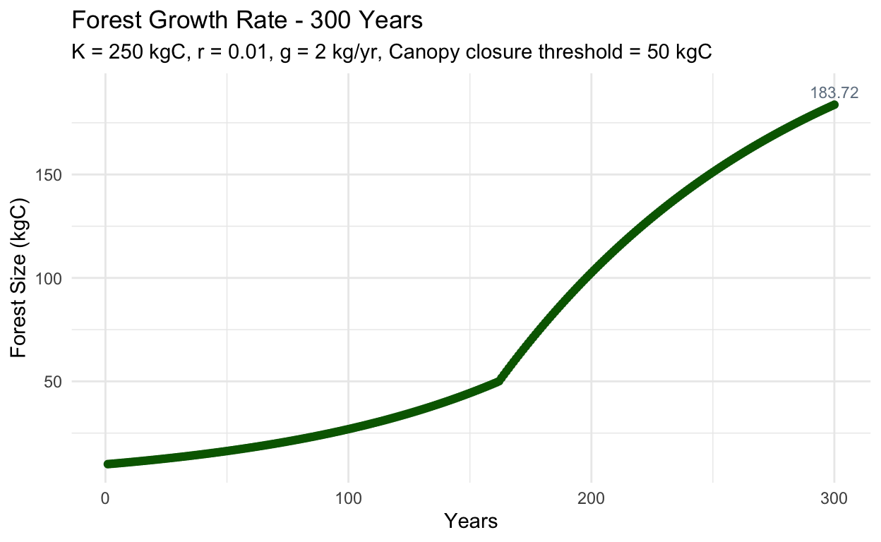
(#fig:ode plot)ODE solver results for forest growth rate model

3.A. Run a sobol sensitivity analysis that explores how the estimated maximum and mean forest size (e.g maximum and mean values of C over the 300 years) varies with the pre canopy closure growth rate (r) and post-canopy closure growth rate (g) and canopy closure threshold and carrying capacity(K)

Assume that parameters are all normally distributed with means as given above and standard deviation of 10% of mean value

# set the number of parameters
np = 200

K = rnorm(mean = K, sd = K*0.10, n = np)
r = rnorm(mean = r, sd = r*0.10, n = np)
g = rnorm(mean = g, sd = g*0.10, n = np)
threshold = rnorm(mean = threshold, sd = threshold*0.10, n = np)

X1 = cbind.data.frame(r = r, K = K, g = g, threshold = threshold)

# repeat to calculate second set of samples
np = 200

K = rnorm(mean = K, sd = K*0.10, n = np)
r = rnorm(mean = r, sd = r*0.10, n = np)
g = rnorm(mean = g, sd = g*0.10, n = np)
threshold = rnorm(mean = threshold, sd = threshold*0.10, n = np)

X2 = cbind.data.frame(r = r, K = K, g = g, threshold = threshold)

# create sobol object and get parameters
sens_forest <- sobolSalt(model = NULL, X1, X2, nboot = 300)

#extract the parameter sets into dataframe
sens_forestSize_df <- as.data.frame(sens_forest$X) 

# Rename the parameters to more meaningful names
sens_forestSize_df <- sens_forestSize_df %>% 
  rename(r = "V1", 
         K = "V2", 
         g = "V3", 
         threshold = "V4")

# Set up wrapper function 
p_wrapper = function(threshold, r, g, K, initialsize, years, func) {
  
  parms <- list(threshold = threshold, r = r, g = g, K = K)
  
  forest_sensitivity <- ode(func = dgrowthrate, y = initialsize, times = years, 
                            parms = parms)
  
  forest_sensitivity <- as.data.frame(forest_sensitivity)
  
  colnames(forest_sensitivity) = c("years","C")

  # calculate the summarizing metric (max and mean carbon values) from the wrapper function
  
  max_carbon <- max(forest_sensitivity$C)
  mean_carbon <- mean(forest_sensitivity$C)

  return(list(max_carbon=max_carbon, mean_carbon=mean_carbon))
}

# Using pmap to run parameter sets into wrapper function
allresults = sens_forestSize_df %>% 
  pmap(p_wrapper, initialsize = initialsize, years = years,
       func = dgrowthrate)

# Extract the results for max and mean carbon values
allres = allresults %>% 
  map_dfr(`[`,c("max_carbon","mean_carbon"))

#Turn the extracted results into format that easier to plot
all_results <- pivot_longer(allres, cols = c(max_carbon, mean_carbon), names_to = "name", values_to = "carbon")

3.B. Graph the results of the sensitivity analysis as a box plot of maximum forest size and a plot of the two Sobol indices (S and T).

# Make boxplot for max and mean carbon values for over 300 years
results_plot <- all_results %>% 
  ggplot(aes(y = carbon, x = name, fill = name)) +
  geom_boxplot() +
  scale_fill_viridis(discrete = TRUE, alpha=0.6) +
  labs(x= "", y = "Carbon (kg)",
       title = "Sobol Analysis - Forest Growth",
       subtitle = "Max & mean values of Carbon over 300 years") +
  theme_minimal() +
  theme(legend.position="none")
  
results_plot

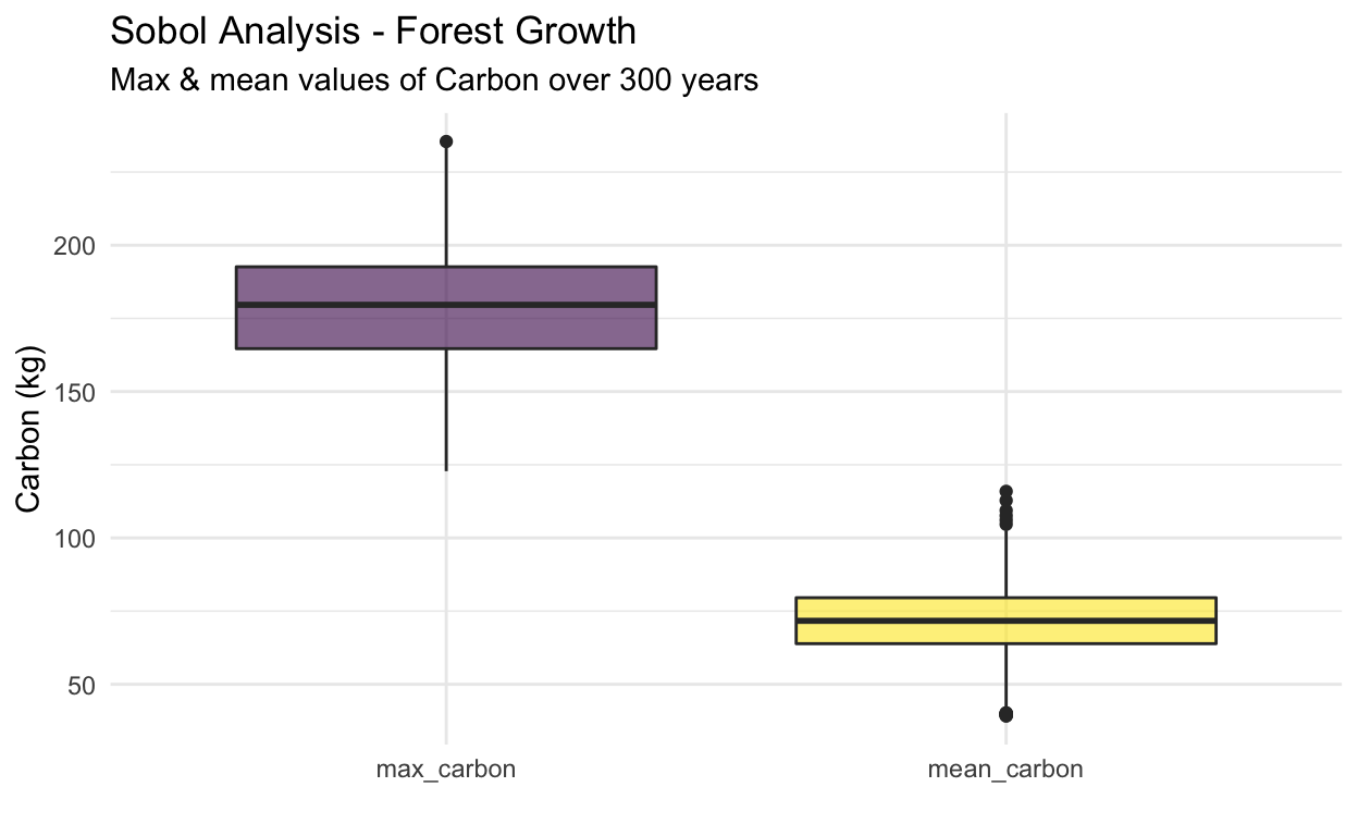
(#fig:box plot)Sobol sensitivity analysis results for forest growth rate model maximum and mean forest size

# Use "tell" to send the mean carbon values over 300 years to sobol analysis
sense_mean <- sensitivity::tell(sens_forest, allres$mean_carbon)

# Calculate the first order sobol indices for mean carbon values over 300 years
sense_mean_S <- as.data.frame(sense_mean$S)

sense_mean_S <- sense_mean_S %>% 
  rowid_to_column(var = "parms")

# Give parameters more meaningful names
sense_mean_S[1,1] <- "threshold"
sense_mean_S[2,1] <- "r"
sense_mean_S[3,1] <- "g"
sense_mean_S[4,1] <- "K"

# Calculate the total effect sobol indices for mean carbon values over 300 years
sense_mean_T <- as.data.frame(sense_mean$T)

sense_mean_T <- sense_mean_T %>% 
  rowid_to_column(var = "parms")

# Give parameters more meaningful names
sense_mean_T[1,1] <- "threshold"
sense_mean_T[2,1] <- "r"
sense_mean_T[3,1] <- "g"
sense_mean_T[4,1] <- "K"

# Use "tell" to send the max carbon values over 300 years to sobol analysis
sense_max <- sensitivity::tell(sens_forest, allres$max_carbon)

# Calculate the first order sobol indecies for max carbon values over 300 years
sense_max_S <- as.data.frame(sense_max$S)

sense_max_S <- sense_max_S %>% 
  rowid_to_column(var = "parms")

# Give parameters more meaningful names
sense_max_S[1,1] <- "threshold"
sense_max_S[2,1] <- "r"
sense_max_S[3,1] <- "g"
sense_max_S[4,1] <- "K"

# Calculate the total effect sobol indecies for max carbon values over 300 years
sense_max_T <- as.data.frame(sense_max$T)

sense_max_T <- sense_max_T %>% 
  rowid_to_column(var = "parms")

# Give parameters more meaningful names
sense_max_T[1,1] <- "threshold"
sense_max_T[2,1] <- "r"
sense_max_T[3,1] <- "g"
sense_max_T[4,1] <- "K"

# Plot the first order sobol indicies for mean carbon values over 300 years

plotSmean <- sense_mean_S %>% 
  ggplot(aes(x = original, y = parms, fill = parms)) +
  geom_col() + 
  scale_fill_manual(values = c("goldenrod2", "indianred1","slateblue3", "darkolivegreen"), 
                    labels = c("Linear Growth Rate", "Carrying Capacity", "Exponential Growth Rate", "Canopy Closure Threshold")) +
  labs(fill = "Parameter", 
       x = "Sobol Sensitivity Value", 
       y = "Parameter",
       title = "First Order Sensitivity Index for Mean Forest Growth") + 
  theme_minimal()

plotSmean

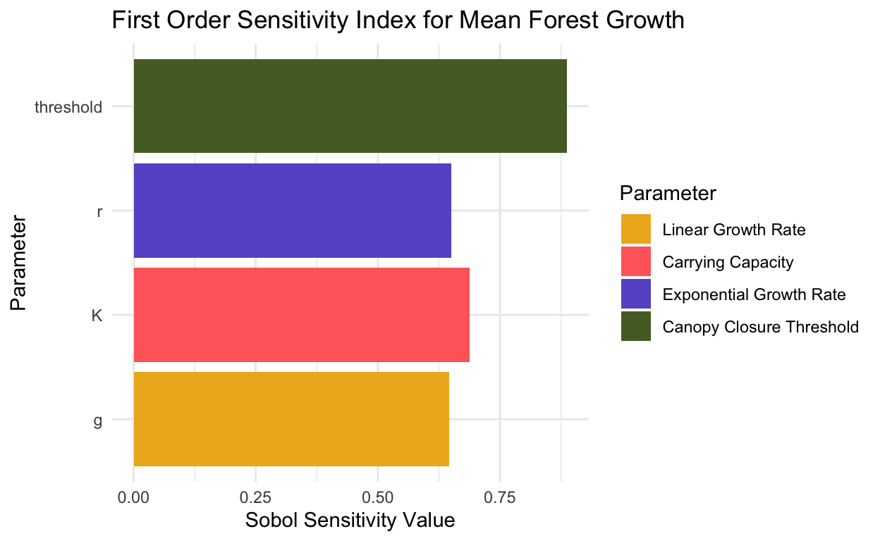
(#fig:plot FOE mean)Mean First Order Effect Sensitivity Index of forest growth

# Plot the first order sobol indicies for max carbon values over 300 years

plotSmax <- sense_max_S %>% 
  ggplot(aes(x = original, y = parms, fill = parms)) +
  geom_col() + 
  scale_fill_manual(values = c("goldenrod2", "indianred1","slateblue3", "darkolivegreen"),
                    labels = c("Linear Growth Rate", "Carrying Capacity", "Exponential Growth Rate", "Canopy Closure Threshold")) +
  labs(fill = "Parameter", 
       x = "Sobol Sensitivity Value", 
       y = "Parameter",
       title = "First Order Sensitivity Index for Maximum Forest Growth") + 
  theme_minimal() 

plotSmax

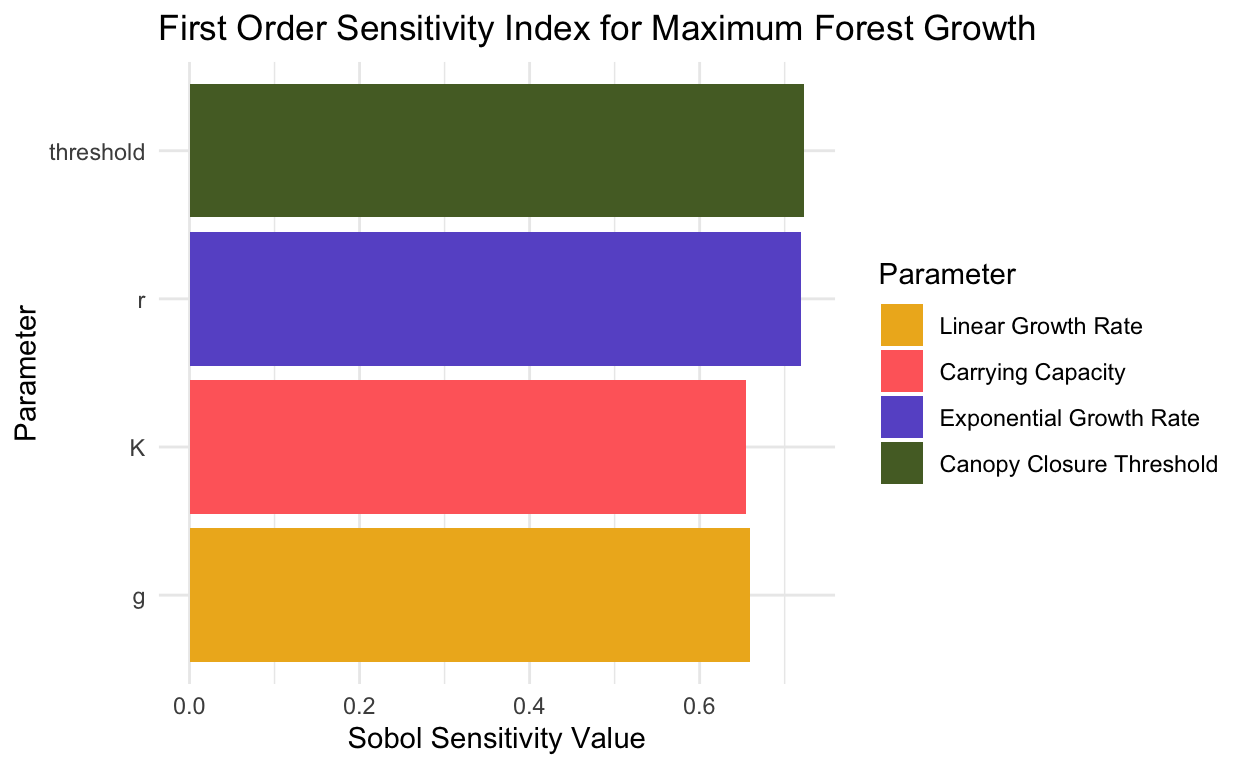
(#fig:plot FOE max)Maximum First Order Effect Sensitivity Index of forest growth

# Plot the total effect sobol indicies for mean carbon values over 300 years

plotTmean <- sense_mean_T %>% 
  ggplot(aes(x = original, y = parms, fill = parms)) +
  geom_col() + 
  scale_fill_manual(values = c("goldenrod2", "indianred1","slateblue3", "darkolivegreen"), 
                    labels = c("Linear Growth Rate", "Carrying Capacity", "Exponential Growth Rate", "Canopy Closure Threshold")) +
  labs(fill = "Parameter", 
       x = "Sobol Sensitivity Value", 
       y = "Parameter",
       title = "Total Effect Sensitivity Index for Mean Forest Growth") + 
  theme_minimal()

plotTmean

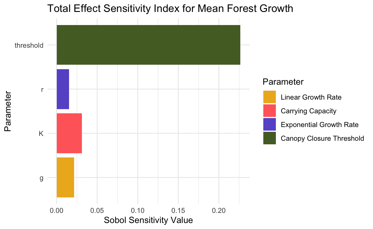
(#fig:plot TE mean)Mean Total Effect Sensitivity Index of forest growth

# Plot the total effect sobol indicies for max carbon values over 300 years

plotTmax <- sense_max_T %>% 
  ggplot(aes(x = original, y = parms, fill = parms)) +
  geom_col() + 
  scale_fill_manual(values = c("goldenrod2", "indianred1","slateblue3", "darkolivegreen"),
                    labels = c("Linear Growth Rate", "Carrying Capacity", "Exponential Growth Rate", "Canopy Closure Threshold")) +
  labs(fill = "Parameter", 
       x = "Sobol Sensitivity Value", 
       y = "Parameter",
       title = "Total Effect Sensitivity Index for Maximum Forest Growth") + 
  theme_minimal() 

plotTmax

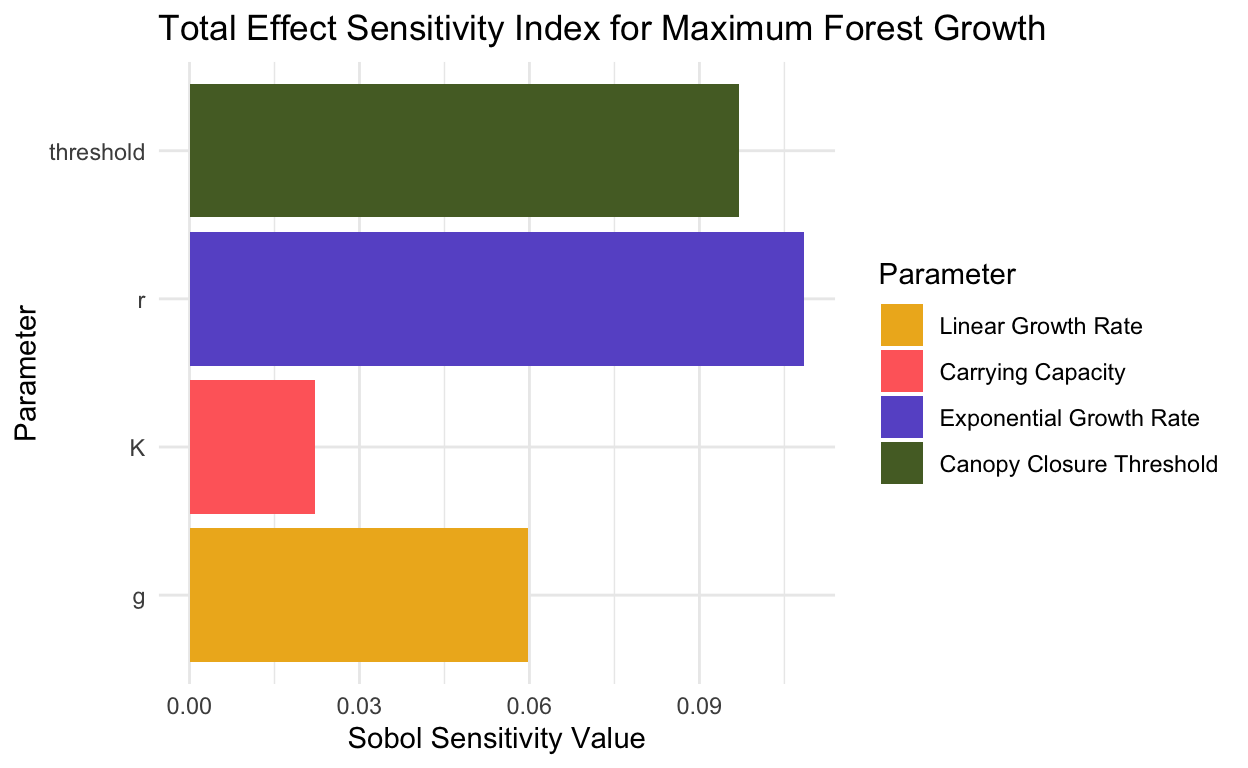
(#fig:plot TE max)Maximum Total Effect Sensitivity Index of forest growth

3.C. Discuss what the results of your simulation might mean for climate change impacts on forest growth

Based on the boxplot of the sensitivity analysis we can see that the max carbon ranges from ~170-190kg with in the IQR. With max and min values of ~245kg and ~120kg respectively. The mean carbon ranging from ~60-80kg within the IQR and with max and min values of ~115kg and ~30kg. This figure and values give insight to understanding how the model will react for mean and max carbon when providing a range of inputs.

The mean first order index shows canopy closure threshold having the greatest sensitivity to change. The maximum first order index follows a similar trend of parameter sensitivity but with diminished differences between parameters. Based on first order index sensitivity we know canopy closure threshold and exponential growth rate hold the most weight in affecting the model.

The mean total effect index indicates that canopy closure threshold will have the greatest impact on model sensitivity. The Max total effect index indicates that canopy closure threshold and exponential growth rate will impact the model the greatest. These trends are similar to the first order index.

When thinking about these results in regards to climate change, we might hypothesis that as average temperatures increase we could see decreased growth in forests. This would affect the canopy closure threshold and growth rate, thus leading to potentially a greater decrease in forest carbon storage.